Eurasian Journal of Business and Economics 2009, 2 (4), 1-26.
Analyzing Regional Variations in Capacity
Utilization of Indian Sugar Industry using
Non-parametric Frontier Technique
Sunil KUMAR
*, Nitin ARORA
**Abstract
Using time series data spanning over the period 1974/75 to 2004/05, this paper provides the trends of capacity utilization (CU) levels in Indian sugar industry from regional perspectives. The results reveal that: i) on an average, the sugar industry in India is operating with the excess capacity in tune to 13 percent in each sampled year; ii) substantial variations in CU levels appear in the sugar industry of 12 major sugar producing states under consideration; iii) a precipitous decline in CU levels is noted in the post-reforms years relative to what has been observed in the pre-reforms period; iv) except the state of Rajasthan, the sugar industry in the remaining 11 states observed a significant decline in CU levels during the post-reforms period relative to the pre-post-reforms period; and v) availability of raw material is most significant variable explaining the CU in Indian sugar industry.
Keywords: Capacity Utilization, Data Envelopment Analysis, Panel Data Tobit-Regression, Indian Sugar Industry
JEL Classification Codes:D24, C61, L66
*
Reader in Economics, Punjab School of Economics, Guru Nanak Dev University, Amritsar-143005 (Punjab), India. Email: [email protected]
**
Introduction
A sugar firm has enough potential to transform the rural economy in its vicinity for the betterment of the people in that area. The transformation takes place through the facilitation of the process of resource mobilization, employment generation (both direct and indirect), income creation, and development of social and physical infrastructure. Recognizing this transformation process, the Indian planners visualized that being a second largest agro-based industry after cotton-textile, the expansion of sugar industry as a principal agro-based industry can tackle a large number of economic tribulations that are present in rural India. The available statistics reveal that sugar industry in India provides direct employment to 0.5 million skilled and unskilled workers and entertains 55 million workers engaged directly or indirectly in sugarcane cultivation, harvesting and ancillary activities (Sanyal et al., 2008). The industry also contributes Rs. 25 billion annually to the center and state exchequer in the form of taxes (ISMA, 2004). Further, with its potential to generate 5000MW surplus power through the process of cogeneration, the industry can ease the energy crisis of Indian economy. In addition, the production of ethanol using molasses (the byproduct of sugar) and blending it with petrol can also help to cut a fraction of rising balance of payments (BOP) deficit due to mounting imports bill for petroleum products.
At present, 453 sugar firms are operating in India and the installed capacity of these mills is ranging between below 1,250 tonnes crushed per day (TCD) of sugarcane and 10,000 TCD. Nevertheless, because of inadequate supply of cane and excessive intervention of the government in fixing the price for both sugar and sugarcane, most of the existing plants and machinery are not being fully utilized in sugar producing states of India. Further, low levels of profitability and low sugar recovery from sugarcane add up the excess capacity in the industry. Besides this, the licensing policy system followed by the government until 1998 did not permit the capacity expansion of the existing mills and thus, restricted them to avail economies of scale. Even after the adoption of delicensing policy of September 1998, the industry is operating with high order of politicization and government control. Consequently, sugar firms are carrying a huge stock of underutilized capital or capacity. Thus, the political control on sugar firms’ operations hinders the techno-economic feasibilities and restricts them to expand their capacity per unit. Contrary to this, sugar industry all over the world has been consolidating and moving towards larger capacity per unit.
(2002) and Ray and Pal (2008)). The existing studies concentrated either on a particular industry or on a set of industries. To the best of our knowledge, no attempt has been made until now to analyze the regional variations in trends of capacity utilization in the Indian sugar industry. The present study is an attempt in this direction and aims to enrich the literature on capacity utilization in Indian industries. In particular, we intend to study the trends in capacity utilization in 12 major sugar producing states of India using the time series data from 1974/75 to 2004/05. For computing the capacity utilization levels, we make use of linear programming based method of data envelopment analysis (DEA). The choice of DEA to compute capacity utilization levels is governed by the fact that it is a non-parametric technique and doesn’t require a priori specification of production function. Also, the information on input prices is not required to obtain the estimates of capacity utilization levels. To check the robustness of the results pertaining to DEA based capacity utilization levels, we also work out capacity utilization levels using traditional minimum capital-output ratio method.
The rest of the paper is organized as follows. Section-II provides a brief overview about the status of Indian sugar industry, especially from regional dimensions. Section-III provides a theoretical overview of the concept of capacity utilization. Section-IV outlines the methodology applied to compute capacity utilization levels in Indian sugar industry. Section-V discusses the construction of relevant input and output variables. Section-VI presents the empirical results pertaining to inter-state variations in the trends of capacity utilization in Indian sugar industry. The final section concludes the paper.
2. Sugar Industry in India: An Overview
Sugar is a highly ‘politicized’ commodity in India and covered under the Essential Commodity Act, 1955. The excessive government participation and control over the industry play a major role in determining the industry’s performance. In Indian sugar industry, the government regulates raw material cost (estimated to account for 75 percent of the operating cost of the sugar manufacturers) and announces a statuary minimum price (SMP) for the purchase of sugarcane by the sugar firms before the start of the sugar year1. Over the years, SMP has followed continuous upward revisions. It has been observed that although SMP serves the political interests of the government but prove to be uneconomical for the sugar firms. Further, the government controls over the supply of sugar and compels the sugar firms to follow a dual price system. Under the ‘levy-sugar quota’, the sugar firms have to surrender a soaring amount of their output to the government at unremunerative prices which are lower than the market-oriented price. However,
the remaining proportion of sugar output can be sold at free market prices without any government restriction.
It is noteworthy that upward revisions in SMP induced only the expansion of area under sugarcane production, and did not provide any incentive to improve the quality of sugarcane in terms of sucrose contents. This is evident from the fact that the sugar recovery content of cane has remained stagnant at around 10 percent for the last two decades as compared with 12 to 13 percent in some other major sugar producing countries.
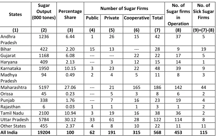
Regarding the structure of sugar industry in India, data for the year 2005 show that there are 20 sugar producing states in India but the combined share of 12 major states is about 97.72 percent. Table 1 provides the following stylized facts of sugar industry in India: i) Among 12 major sugar producing states, the sugar firms of Uttar-Pradesh (UP) and Maharashtra are contributing about 27.06 percent and 30.12 percent, respectively to the total sugar production of India.
Table 1: Some Stylized Facts about Sugar Industry in India as on 30/9/2005
Number of Sugar Firms States
Sugar Output (000 tones)
Percentage
Share Public Private Cooperative Total
No. of Sugar firms
in Operation
No. of Sick Sugar
Firms
(1) (2) (3) (4) (5) (6) (7) (8) (9)=(7)-(8)
Andhra Pradesh
1236 6.44 1 26 15 42 37 5
Bihar 422 2.20 15 13 --- 28 9 19
Gujarat 1168 6.08 --- --- 22 22 17 5
Haryana 409 2.13 --- 3 12 15 14 1
Karnataka 1950 10.15 3 23 22 48 39 9
Madhya Pradesh
94 0.49 2 4 5 11 8 3
Maharashtra 5197 27.06 --- 21 165 186 142 44
Orissa 45 0.23 --- 5 3 8 6 2
Punjab 338 1.76 --- 7 16 23 19 4
Rajasthan 6 0.03 1 1 1 3 1 2
Tamil Nadu 2100 10.94 3 19 16 38 36 2
Uttar Pradesh 5784 30.12 33 61 28 122 114 8
Other States 455 2.37 4 8 10 22 11 11
All India 19204 100 62 191 315 568 453 115
Sources: i) Handbook of Sugar Statistics, September 2006, Indian Sugar Mills Association, New Delhi; and ii) Indian Sugar Year Book 2005/06, Indian Sugar Mills Association, New Delhi.
shut down their operations. Thus, the installed capacity of one-fifth sugar firms is remained underutilized; and iii) Sugar firms in India are operating under three types of ownership structures viz., public, private and cooperative sectors. The cooperative sector dominates with the 315 cooperative sugar firms. It is apparent from the data that 55.46 percent of sugar firms are operating under the cooperative sector as compared to the 33.63 percent under private ownership and 10.92 percent under public ownership.
3. Concept of Capacity Utilization: Theoretical Underpinnings
Capacity is a short-run concept, for which firms and industry face short-run constraints, such as the stock of capital or other fixed inputs, existing regulations, the state of technology and other technological constraints (Morrison, 1985). However, measuring the rate of capacity utilization requires identifying the capacity output Y*. The capacity utilization rate is then defined as the ratio of the actual output Y0 to capacity output, i.e.,
0 * Y CU
Y
=
where, capacity output (Y*) can be defined as the potential output level in the short run and capacity utilization (CU) is the ratio of actual output to potential output (Kirkley et al., 2002). However, the notion of capacity output has been defined in two alternative ways; i) physical or engineering concept; and ii) an economic concept. As per the physical or engineering concept, the potential output may be technologically derived and hence defined relative to the maximum possible physical output that the fixed inputs are capable of supporting when the variable inputs are fully utilized (Johanson, 1968). Alternatively, full capacity output is that level of output, which the existing stock of equipment is intended to produce under normal conditions with respect to the use of variable inputs (Smithies, 1957). In contrast, economic concept measure the full capacity output of the firm at the point where average cost is minimum (Chamberlin, 1947). Thus, from the point of view of an economist, the potential output can be defined relative to an economic optimum such as the level of output, which minimizes cost or maximizes revenue or profits (Gréboval and Munro, 1999). Figure 1, presents two notions of capacity output elaborated through the engineering based and economic definitions of capacity. Panel A explains OYo level of capacity output as per the engineering concept of capacity whereas, in Panel B, OYE is the economic
economists’ concept (Budin and Paul, 1961). Most of the managers and technical experts prefer to operate with the engineering definition of capacity and incidentally the same definition is the basis of the capacity definition of Central Statistical Organization (CSO), Ministry of Statistics and Program Implementation, India (Paul, 1974). Further, empirical determination of the economists’ version of capacity output is indeed difficult especially in the context of multiproduct firm. However, if most cost curves are L-shaped, the economic concept can also be approximated by the engineering concept of capacity (Johanston, 1960).
Figure 1: Two Concepts of Capacity Output
Source: Grèboval, (2002)
with existing plant and equipment, provided the availability of variable factor of production is not restricted. Thus, capacity utilization is the degree to which the decision making unit (DMU)2 is achieving its potential (capacity) output given its physical characteristics (i.e. fixed inputs such as fixed capital in our case). In contrast, technical efficiency is related to the difference between the actual and potential output given both fixed and variable input use. A DMU may be operating at below its capacity level due to underutilization of the fixed inputs, or the inefficient use of these inputs, or some combination of the two. The two concepts are illustrated in Figure 2, in which a DMU of a given size is observed to be producing Oo level of output as a result of using Vo levels of inputs.
Figure 2: Capacity Utilization and Technical Efficiency
Source: Food and Agriculture Organization, (2008)If all inputs were fully utilized (i.e. using Vc rather than Vo variable inputs), and the
DMU was operating at full efficiency, then the potential (capacity) output would be Oc. Even at the lower level of input usage, if the DMU was operating efficiently it
would be expected to produce OE level of output. Hence, the difference Oc - OE is
due to capacity underutilization; and the difference OE - Oo is due to inefficiency.
2
4. DEA based Capacity Utilization Model
The DEA approach derives a deterministic production frontier describing the most technically efficient combination of outputs, given the state of technology, fixed and variable inputs. Färe (1984) introduced his methodology as a means of measuring the technological-economic concept of capacity and CU for manufacturing firms, and further developed by Färe et al. (1989). The DEA approach calculates capacity output, given the variable factors are unbounded and fixed factors, and state of technology constraint output. Capacity output corresponds to the output that could be produced, given full and efficient utilization of variable inputs and given the constraints imposed by the capacity base i.e., the fixed factors, the state of technology, environmental conditions and resource stock. In practice, because the data reflect both technological and economic decisions made by firm, the variable inputs correspond to full and efficient utilization under normal operating conditions.
The mathematical model to compute capacity measure, proposed by the Färe et al. (1994) can be defined as follows:
{t, , }
tn
Maximize (1)
Subject to: ,
,
,
′ ≤
′
≥ ∈
′
= ∈
i t
t t
tm m X
tn n X
y Y
x X m F
x X n V
φ λ µ
φ
φ
λ
λ
µ
λ
, 0.
≥ t
λ µ
Where,
φ
ti= capacity measure at time t for ith decision making unit (DMU). Assumethere are m fixed inputs, n variable inputs and k outputs, then xtm, xtn and ytk
denotes, respectively, the fixed input, variable inputs and output vectors for the tth year. Thus, xtm is a (m×1) column vector, xtn is a (n×1) column vector and ytk is a
(k×1) column vector. Moreover, Xm=
(
x x1, 2,...,xm)
is the(m T× )matrix of fixedinputs,Xn=
(
x x1, 2,...,xT)
is the (n T× ) matrix of variable inputsandY =
(
y y1, 2,...,yT)
is the k T× output matrix. Further, λ is vector of intensityvariable of orderT×1 andµtnrepresents input utilization rate of variable input n at
(
)
i
i t
DEA t i
t
CU
θ
φ
=
(2)
Where,
θ
ti=Technical efficiency score for the ith DMU at time t andφ
ti=capacitymeasure for the ith DMU at time t. The
θ
ti can be defined from the followingmodel which is popularly known as output-oriented CCR model.
{o, }
Maximize
(3)
Subject to:
,
,
0.
′
≤
′
≥
≥
i t
t t
t
y
Y
x
X
φ λ
θ
θ
λ
λ
λ
In model (3) the output constraint is same as given in model (1) whereas, the handling of input constraints differs to some extent. In model (3), each input acquires same treatment and no differences exist between fixed and variable
inputs. Thus, X =
(
x x1, 2,...,xT)
becomes a matrix of order(
m+ ×n)
T. It is evident from relation (2) that capacity utilization and technical efficiency are related with each other. We made use of relationship (2) to compute the levels of capacity utilization in the 12 major sugar producing states of India.However, the DEA approach has some limitations: i) it is a non-statistical approach, which makes statistical tests of hypothesis about structure and significance of estimates difficult to perform; ii) because DEA is non-statistical, all deviations from the frontier are assumed to be the result of inefficiency; iii) estimates of capacity and capacity utilization may be sensitive to the particular data sample (a feature shared by the dual cost, profit or revenue function approach). Thus, to check the robustness of results obtained from DEA based method, we also computed CU levels using traditional minimum capital output ratio method. The method of minimum capital output ratio, as suggested by the National Conference Board of the United States, estimate capacity using capital output ratio. Fixed capital output ratios are estimated in terms of constant prices. A benchmark year is then selected on the basis of the observed lowest capital output ratio. In choosing the benchmark year, other independent evidence is also taken in to consideration. The lowest observed capital output ratio is considered as capacity output. The estimate of capacity is obtained from real fixed capital stock deflated by minimum capital output ratio. The utilization rate is given by actual output as a proportion of the estimate of capacity.
Thus,
(
)
i t ˆ 100T t
Y CU
K
= ×
ˆ t t
t
K K Min
K Y
=
Where,
(
T)
it
CU is capacity utilization by ith state at time t, 'Yt’ is gross output, Kˆ
is the estimate of capacity, ‘K’ represents real gross fixed capital, and
(
K Yt t)
represents capital output ratio. Although, this method provides useful measure of capacity utilization, the problems of measurement of capital are formidable. Capital is even more difficult to measure than capacity. Needless to say, the usefulness of this method depends critically on accuracy of the measurement of capital.
5. Database and Measurement of Variables
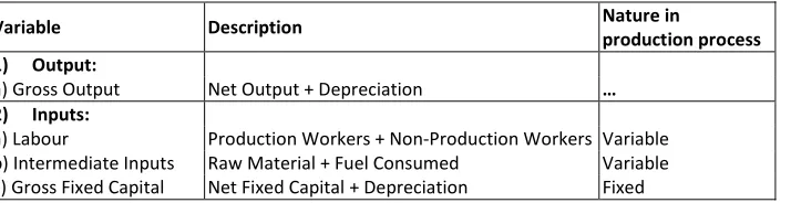
Our empirical analysis is confined to the period of 31 years from 1974/75 to 2004/05, which has been further divided into two sub-periods on the basis of changes in macroeconomic policy governing the Indian economy: i) Pre-reforms period (1974/75 to 1990/91); and ii) Post-reforms period (1991/92 to 2004/05). The required data have been provided by the ‘Annual Survey of Industries (ASI)’ wing of Ministry of Statistics and Programme Implementation (MOSPI), Government of India, on the payment basis. The foremost requirement for computing CU levels in the sugar industry of 12 major sugar producing states is to specify a set of input and output variables. Our set of variables includes single output variable and three input variables. A detailed description of these variables is given in Table 2. Except labour, all the variables have been deflated by using suitable price indices3.
Table 2: Description of Variables for Calculating CU Levels
Variable Description Nature in
production process 1) Output:
a) Gross Output Net Output + Depreciation …
2) Inputs:
a) Labour Production Workers + Non-Production Workers Variable b) Intermediate Inputs Raw Material + Fuel Consumed Variable c) Gross Fixed Capital Net Fixed Capital + Depreciation Fixed
Source: Authors’ Elaboration
3
However, to generate a series of gross fixed capital stock, we followed the popular perpetual inventory method. This requires a gross investment series, an asset price deflator, a depreciation rate, and a benchmark capital stock. We adopted the following 3-steps procedure to obtain a series of gross fixed capital stock at constant prices.
Step 1: For constructing a series of gross fixed capital stock, the most important prerequisite is the figure of capital stock in the benchmark (initial) year i.e., K0 . To
obtain K0, we assume that the value of finished equipment of a balanced age
composition would be exactly half the value of equipment when it was new. Hence, in the present analysis, twice the book value of fixed assets in the benchmark year at 1981/82 prices, has taken as an estimate of the replacement value of fixed capital i.e., K0 =2×B0 (where B0 is the book value of fixed capital net of the
depreciation in the benchmark year). Banerji (1975), Roychaudhury (1977), Goldar (1986), Sarma and Rao (1990), Singh and Ajit (1995), Kumar (2001), and Sharma and Upadhyay (2008) have followed this approach to reach at the figure of fixed capital stock for the benchmark year in their empirical research works.
Step 2: After obtaining the estimate of K0, we obtained the series of gross real investment (It) by using the following relationship:
1 t t t t
t
B B D
I P
−
− +
=
where Bt =Book value of fixed capital in the year t, Dt =Value of depreciation of
fixed assets in year t, and Pt=Implicit deflator for gross fixed capital formation for
registered manufacturing sector in National Accounts Statistics (NAS).
Step 3: Given the estimate of K0 and the series of It, the following relationship has
been used to construct a series of gross fixed capital stock at 1981/82 prices:
1 1
t t t t
K =K− + −I dK−
where Kt=Gross fixed capital at 1981-82 prices in the year t, It=Gross real
investment in the year t, and d=Annual rate of discarding of capital. Following Unel (2003), we have taken the annual rate of discarding of capital equals to 5 percent.
that it imposes fewer restrictions on the production technology4. In addition, this reduces the effects of random noise due to measurement errors in inputs and output(s).
6. Empirical Results
This section presents the empirical results pertaining to the trends in CU over the entire study period and distinct sub-periods. Both DEA-based and traditional measures of CU have been obtained for 12 major sugar producing states along with All-India level5. We note that leaving the case of Karnataka, the coefficient of correlation between CUDEA and CUT are both positive and statistically significant in
all major sugar producing states of India (see Table 3). Thus, we can safely infer that our DEA-based results are quite robust. Therefore, in the rest of the analysis, we concentrate on the trends in CUDEA measure.
From Table 3, we observe that during the entire study period, the value of CUDEA
measure for All-India level varied between 0.61 and 1, with an average of 0.87. This indicates that in each year of the study, the level of CU, on an average, is about 87 percent in Indian sugar industry. Thus, the average amount of excess capacity in Indian sugar industry is about 13 percent in the each year of the study period. The year-wise analysis reveals that the CUDEA measure achieved its maxima in the year
1982/83 and minima in 2004/05, and exhibited a precipitous decline in the post-reforms years (see Figure 3). Turning to the comparative analysis of average CUDEA
measure between the sub-periods6, we note an increase in the average excess capacity in the post-reforms period by about 15 percentage points relative to what has been observed in the pre-reforms period. This is evident from the fact that mean CUDEA has declined from 0.945 for the first sub-period to 0.788 for the second
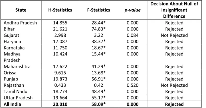
sub-period period (see, Table 3). In addition, the results of Kruskall-Wallis test showed that observed decline in CU levels in the post-reforms period is statistically significant (see Table 4).
4
The firm level input-output pairs are feasible, although not individually reported. Therefore, by the assumption of convexity, the average output bundle will always be feasible. The aggregate input-output bundle will be feasible only under the condition of non-additivity of technology (Ray, 2002). 5
The figures of CU for the sugar industry of All-India have been obtained via using the sum of the outputs and sum of each input of 12 sugar producing states as the measure of its output and inputs, respectively.
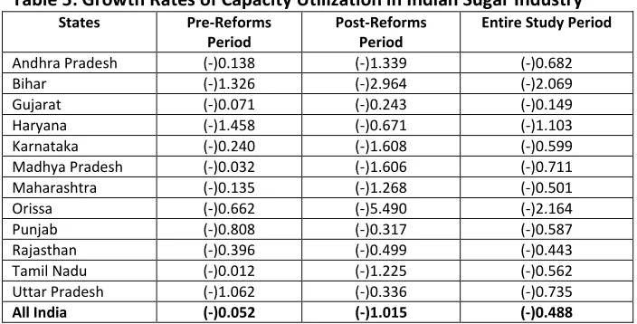
The perusal of growth rates7 of CU in Table 5 confirms that capacity utilization has followed a path of deceleration during the entire study period (a growth rate of -0.488 percent per annum reflects this). The comparison of growth rates in CU levels during the sub-periods also revalidates our above drawn inference that capacity utilization declined swiftly in the post-reforms years. Here, we note that capacity utilization declined at a rate of -1.075 percent per annum during the post-reforms period in comparison of -0.052 percent in the pre-reforms period. In the nutshell, we can safely infer that the excess capacity in Indian sugar industry has increased sharply during the post-reforms period. Therefore, a meticulous inspection of the causes of such a drastic change in CU levels in the post-reforms period is needed.
7 The growth rates of capacity utilization for individual states and aggregated Indian sugar industry during the period 1974/75 to 2004/05 have been estimated from the following semi-log equation which takes the form:
logCUDEAt = + +φ λ εt (8) Where,
t
DEA
CU represents capacity utilization at time period t and ε is the white noise error term.
The growth rates for the period 1974/75 to 2004/05 have been obtained as
[
exp( ) 1 100λ − ×]
. However, the impact of industrial liberalization on CU trends has been captured by computing the growth rates for these sub-periods on the basis of a linear spline function which has been developed by Poirier (1974) and applied by Goldar and Seth (1989), Seth and Seth (1994), Pradhan and Barik (1998) and Kumar (2001). Assuming that there are two sub-periods, two equations are needed to be formulated which takes the following forms:Sub Period 1: log 1 1 1
t
DEA
CU = +φ λt+ε When t < t1 (9)
Sub Period 2:
2 2 2
log
t
DEA
CU = +φ λt+ε When t ≥ t1 (10)
where t1 and t2are the points of structural breaks. In order to tackle the discontinuities in the sub-period
wise growth rates, the linear spline function is reparametrized as: log 1 1 2 2
t
DEA t t
CU = + ∂ϕ w + ∂ w +ε (11)
Where, w1t =t
and 1
2
1 1
0 if t<t
if t t
t
w
t t
=
− ≥
The growth rate for the ithsub-period can be derived by
[
exp( ) 1λ
i − ×]
100and λis are obtained as1 1
Figure 3: Trends of Capacity Utilization in Indian Sugar Industry
Table 4: Results of Kruskal-Wallis Test
State H-Statistics F-Statistics p-value
Decision About Null of Insignificant
Difference
Andhra Pradesh 14.855 28.44* 0.000 Rejected
Bihar 21.621 74.83* 0.000 Rejected
Gujarat 2.998 3.22 0.084 Not Rejected
Haryana 17.087 38.37* 0.000 Rejected
Karnataka 11.750 18.67* 0.000 Rejected
Madhya Pradesh
10.424 15.44* 0.000 Rejected
Maharashtra 17.622 41.29* 0.000 Rejected
Orissa 9.615 13.68* 0.000 Rejected
Punjab 19.873 56.91* 0.000 Rejected
Rajasthan 0.433 0.42 0.520 Not Rejected
Tamil Nadu 18.773 48.49* 0.000 Rejected
Uttar Pradesh 19.664 55.17* 0.000 Rejected
All India 20.010 58.09* 0.000 Rejected
Table 5: Growth Rates of Capacity Utilization in Indian Sugar Industry
States Pre-Reforms Period
Post-Reforms Period
Entire Study Period
Andhra Pradesh (-)0.138 (-)1.339 (-)0.682
Bihar (-)1.326 (-)2.964 (-)2.069
Gujarat (-)0.071 (-)0.243 (-)0.149
Haryana (-)1.458 (-)0.671 (-)1.103
Karnataka (-)0.240 (-)1.608 (-)0.599
Madhya Pradesh (-)0.032 (-)1.606 (-)0.711
Maharashtra (-)0.135 (-)1.268 (-)0.501
Orissa (-)0.662 (-)5.490 (-)2.164
Punjab (-)0.808 (-)0.317 (-)0.587
Rajasthan (-)0.396 (-)0.499 (-)0.443
Tamil Nadu (-)0.012 (-)1.225 (-)0.562
Uttar Pradesh (-)1.062 (-)0.336 (-)0.735
All India (-)0.052 (-)1.015 (-)0.488
Note: All the figures calculated using CUDEA measure of capacity Utilization.
Source: Author’s Calculations
The DEA-based capacity utilization method also supplies rich diagnostic informations that can be used, at least theoretically, to know the causes of excess capacity and recommend how to vanish the scenario of the excess capacity in the industry. The information on µtnin model 1 may be used for this purpose. The
tn
µ represents input utilization rate of variable input n at time t, and is defined as the ratio of the optimal use of each input to its actual usage. A value of µtnequals
to 1.25 (say) indicates that the variable input n should be increased by 25 percent in the year t so as to achieve the full capacity output corresponding to the best-practice frontier. Converse implies for any value less than 1. Table 6 provide the average estimates of adjustment needed in the usage of variable inputs during the entire study period and two sub-periods, so that the level of full capacity output can be achieved in Indian sugar industry.
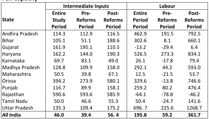
Table 6 provides that a representative sugar mill in India, on an average, need 46.04 percent more intermediate inputs and 195.81 percent more labour inputs to operate on full capacity. Further, on an average, necessary requirement of variable inputs to mitigate the excess capacity in the sugar industry has increased during the post-reforms period relative to what needed in the pre-reforms years8. It is well known fact that the acute shortage of sugarcane, the basic raw material which accounts about 80 percent weight in intermediate inputs given the self sufficiency of sugar mills in its energy requirements, is the main factor which compels the
8
several mills to cease their operations even in the mid of the peak season and, thus, restrict them to operate on full capacity. It is significant to note here that the sugarcane shortage is countrywide phenomenon and not limited to a particular state. Regarding labour input, we note that a huge adjustment to labour input is required to achieve capacity output. Such a huge amount is not surprising given an acute shortage of sugarcane, which discontinues the working of sugar firms even during the peak season. It is worth mentioning here that with rising slack of intermediate inputs during the post-reforms period, the slack of labour force has also increased. This indicates that if Indian sugar industry operates at full capacity then there is huge possibility to increase employment in this industry both directly and indirectly9.
Table 6: Percentage Adjustment Needed in Variable Inputs to Operate on
Full Capacity
Intermediate Inputs Labour
State
Entire Study Period
Pre- Reforms
Period
Post- Reforms
Period
Entire Period Period
Pre- Reforms
Period
Post- Reforms
Period
Andhra Pradesh 114.3 112.9 116.5 462.9 191.5 792.5
Bihar 105.1 51.1 188.6 302.6 8.1 660.1
Gujarat 161.9 195.1 110.5 -13.2 -29.4 6.4
Haryana 162.2 144.0 190.3 526.5 273.3 834.1
Karnataka 69.7 83.1 49.0 26.1 -17.8 79.4
Madhya Pradesh 128.8 109.9 158.0 292.1 44.2 593.0
Maharashtra 50.5 39.8 67.1 12.5 -21.5 53.7
Orissa 394.2 273.9 580.1 329.6 -13.8 746.6
Punjab 116.7 89.9 158.1 259.2 80.2 476.4
Rajasthan 590.6 593.6 585.9 -64.1 -78.8 -46.2
Tamil Nadu 50.0 46.6 55.3 50.4 -24.7 141.6
Uttar Pradesh 135.3 109.4 175.2 696. 7 225.6 1268.7
All India 46.0 39.4 56. 4 195.8 59.2 361.7 Source: Authors’ Calculations
6.1. Inter-State Analysis
Table 3 also presents year-wise CU levels in 12 major sugar producing states of India. We note that the average CU levels range between 0.35 for Rajasthan and 0.88 for Maharashtra, and in two states, namely, Maharashtra and Karnataka, these levels are found to be above All-India level. Further, baring the sugar industry of Rajasthan (where average CU levels remained almost invariant in the sub-periods), the sugar industry in remaining states observed a decline in average CU levels during the post-reforms period relative to that of the pre-reforms period.
9
The results of Kruskal-Wallis test brought that, except the states of Gujarat and Rajasthan, the decline in average CU levels in remaining states is statistically significant (see Table 4). Turning to the analysis of growth rates of CU levels, we note that CU levels followed a negative trend in all the states. Except Bihar, Orissa, and Haryana, the sugar industry in remaining 9 states followed a regress in CU levels at a rate more than 1 percent per annum. The comparative analysis of growth rates in CU levels between the pre- and post-reforms years reveals that except Punjab, Haryana and Uttar Pradesh, the rate of decline in CU has been observed to be relatively higher in second sub-period (see Table 5). In sum, we can safely infer that leaving a few exceptions, the excess capacity in sugar mills followed an ascent in a majority of sugar producing states.
Table 6 also provides necessary requirements at state levels in variable inputs to realize full capacity output and reveals that: i) for all the states a huge increase in intermediate inputs, between the range of 50.036 percent for Tamil Nadu and 590.571 percent for Rajasthan, is required to operate on full capacity during the entire study period; ii) except two states, namely, Gujarat and Rajasthan, the remaining 10 states have potential to increase the labour input so as to operate at full capacity10; iii) except the states of Karnataka and Rajasthan, each state has exhibited a potential increase in the intermediate inputs requirement during the post-reforms period as compare to the pre-reforms period; and iv) the potential labour requirements have increased for all states during the post-reforms period11.
On the whole, the aforementioned analysis confirms a decline in CU levels in Indian sugar industry over the entire study period and distinct sub-periods. This decline is primarily driven by: i) acute shortage of sugarcane at farm level, which primarily occurred because of mounting sugarcane arrears to be paid to the farmers by the sugar mills. The untimely payments for sugarcane by the sugar firms compel the farmers to diversify and produce even less remunerative crops such as wheat and rice, for which assured marketing is available; and ii) inability of sugar firms to purchase the sugarcane at remunerative price. Nevertheless, the statuary minimum price (SMP) announced by government is always high enough and unconnected with the market oriented price of sugarcane. It adds up the variable cost of production and, thus, sugar firms shut-down their operations even during the mid of the peak seasons.
10
In two states namely, Gujarat and Rajasthan, labour has been observed to be over utilized during the entire study period and thus, call for the reduction of the workforce by 13.23 percent and 64.10 percent, respectively.
11
6.2. Factors Explaining Variations in Capacity Utilization
In the above analysis, we note that CU estimates differ substantially across Indian states. However, their differences may occur because of a variety of factors such as access to technology, structural rigidities, differential incentive systems, level of profitability, etc. In applied research, we often rely on regression analysis to examine the influence of environment factors on capacity utilization. Unfortunately, the simple linear regression model is not appropriate in the present context, because the range of CU levels (dependent variable) is (0,1] and, therefore, estimation of the model using ordinary least square procedure may produce biased estimates if there is a significant position of the observations equal to one (Resende, 2000). In such cases, the appropriate regression model is known as a Tobit or Censored regression model which handles data that is skewed and truncated (Avkiran, 1999). For modeling the effect of environmental factors on capacity utilization, we used both fixed effect and random effect Tobit models. The one way fixed effect panel data Tobit model for observation (state) i at time t can be defined as follows:
*
1 1
* *
, if 1, a n d (1 2 ) 1, o t h e rw is e
it
N k
j
i t j ij j i t
j j
i t it it i t
y z x
y y y
y α β ε = = = + +
= <
=
∑
∑
where, zij=1 if i=j and 0 elsewhere and
ε
it~IIN(0,σ
ε2) . However,it
j
x represents
the jth explanatory variable and βj are corresponding parameters. The yit* is a
latent variable andyitis the dependent variable. The joint probability function or
likelihood function can be written as:
1 1 1
( , , / , , , , , ),( , ) ( / , , , )
T
i iT i iT i iT j j it it ij j j it
t
f y y x x z z
α β
f y x zα β ε
d∞
−∞
=
K K K
∫
∏
(13)
where,
2 1 1 2 1 2 2 1 /( , ), ( , ) 2 N k j it j ij j it
j j
y z x
it it it j j
f y x z e ε
α β σ ε α β σ = = − − − ∑ ∑ = Π
,
Ify
it<1
and,
1 it 1
k N
j
j j ij
j j e x z β α φ σ = = + =
∑
∑
,
Ify
it
=1
*
1
* *
, if 1, (1 4 )
1,
it
k j
i t j i i t
j
i t it it
i t
y x v
y y y a n d
y o th e r w is e
β µ = = + +
= <
=
∑
where, µi~IIN(0,σµ2)and
2
~ (0, )
it v
v IIN σ are assumed to be independent of
xi1,…,xiT . Using f as generic notation for a density or probability mass function, the likelihood function for model (14) can be written as:
(
(
1,
,
/
1,
,
),
)
(
/
,
,
) (
)
T
i iT i iT j it it i j i i
t
f
y
y
x
x
β
f y
x
µ β
f
µ µ
d
∞
−∞
=
∫
∏
K
K
(15)where, 2 2 1 2 2
1
(
)
2
i if
e
µµ σ µ
µ
σ
−=
Π
,
and,
(
)
2 1 2 1 2 , 2 1 ( / ), 2 k j it jit i
j v
y x
it it i j
v
f y x e
β µ σ
µ β
σ
= − − − ∑ = Π,
If
y
it<1
1 it k j j i j v x β µ φ σ = + =
∑
,
Ify
it
=1
Note that the later two expressions are similar to the likelihood contribution in the fixed effect case. The only difference is the inclusion of µi in the conditional mean. The parameters of models (12) and (14) can be estimated via applying the method of maximum likelihood using likelihood functions (13) and (15), respectively. In present study, we used STATA Version 10 to estimate the parameters by the method of maximum likelihood.
levels. The variable RETURN is defined as the ratio of contribution of capital12 to gross fixed capital. The variable RETURN is used as a proxy for the level of profitability in the industry. We hypothesize that profitability has a positive relationship with the CU levels i.e., higher profitability acts as an incentive to exploit the available capacity up to its optimum extent, and vice-versa. The variable SKILL represents the availability of human skills and highlights the availability of the trained manpower including supervisory, administrative and managerial staff. Following Ghosh and Neogi (1993) and Kumar and Arora (2007), it has been measured as the ratio of skilled persons (i.e., all employees minus production workers) to all employees. We also hypothesize that SKILL affect CU levels positively. The variable raw material (RMATERIAL) represents quantity of sugarcane crushed by each state at given point of time. This variable has also been expected to affect CU levels positively.
Table 7 provides the results of Tobit regression models. The statistical significance of Fishers’ specification test (ANOVA F-Statistics) in fixed effect model and Lambda-Max (LM) and likelihood-ratio (LR) tests in random effect model advocate the use of these panel data models over the pooled OLS estimators. Both fixed and random effect models reject the null hypothesis regarding insignificant individual state effect. Further, it has been observed that there exists a diminutive difference between the magnitude of the coefficients obtained from both fixed and random effect models. Both models also report same direction of the impacts of explanatory variables on the CU levels in Indian sugar industry.
From Table 7, we note that barring the explanatory variable SKILL, all other variables are significantly affecting the CU levels in Indian sugar industry. The variable RMATERIAL bears a sign in agreement with a-priori expectations, and thus found to be positively affecting capacity utilization. The direct connotation of this result is that with the falling levels of the availability of sugarcane, the CU levels in Indian sugar industry are falling. We, therefore, recommend that efforts must be taken to enhance the supply of sugarcane to realize the full capacity in terms of sugar industry of India. Further, the variable (K/L) is bearing a negative impact on CU in Indian sugar industry. The negative impact of increasing capital intensity (K/L) shows that increasing stock of capital per unit of labour will add up the already rising excess capacity due to lack of the availability of raw material (i.e., sugarcane). Moreover, a negative and statistically significant coefficient of RETURN does not support our inference about the positive impact of it on CU levels. The customary environment of persistence losses in the industry might have discouraged the producers to react and extend capacity utilization despite of an improvement in RETURN.
12
Table 7: Results of Fixed- and Random-Effect Tobit Regression Model
Fixed Effect Model Random Effect Model Explanatory Variables
(Parameters) Coefficient Z-value p-value Coefficient Z-value p-value
Constant
( )
β1 0.526* 9.480 0.000 0.710* 11.32 0.000Skill
( )
β2 0.009 0.110 0.914 1.191 0.230 0.819 K/L ( )3
β (-)1.61e-06* (-)19.280 0.000 (-)1.60e-06* (-)18.88 0.000
RETURN
( )
β4 (-)0.014* (-)5.090 0.000 (-)0.014* (-)5.100 0.000RMATERIAL
( )
β5 1.93e-09* 8.820 0.000 (-)0.014* 8.690 0.000Fisher Specification Test
1
0
N j j
Null α =
=
∑
86.68* --- 0.000 --- ---
LM-Test (Null σμ=0) --- --- --- 0.189* --- 0.000
LR-Test (Null σμ =0) --- --- --- 398.910* --- 0.000
Note: * indicates that null hypothesis is rejected and parameter is significant at 5 percent level of significance.
Source: Author’s Calculations
7. Conclusions and Policy Implications
Using time series data of 31 years spanning over the period 1974/75 to 2004/05 for 12 major sugar producing states of India, the present study aims to analyze the inter-state variations in capacity utilization in Indian sugar industry. The linear programming based data envelopment analysis (DEA) has been used for computing CU measures. The major findings of the study are: i) the average amount of excess capacity in Indian sugar industry is about 13 percent in the each year of the study period; ii) excess capacity increased significantly by about 15 percent in the post-reforms period (1991/92 to 2004/05) relative to the pre-post-reforms period (1974/75 to 1990/91); iii) The CU levels followed a path of deceleration (as ascertained by negative growth rates) during the entire study period and the deceleration become more noticeable during the post-reforms period; iv) at full capacity level, 46.04 percent of more intermediate inputs and 195.8 percent of more labour are needed, which indicates that, reaching at full capacity would surely increase the employment in the industry; v) except the states of Karnataka and Rajasthan, each state has exhibited potential increase in intermediate inputs requirement during the post-reforms period as compare to the pre-reforms period; vi) the potential labour requirement has increased for all states during the post-reforms period; vii) an increase in capital-intensity adds up the existing excess capacity in the industry; and viii) the availability of raw material is a major determinant of capacity utilization.
sugarcane by sugar mills, and b) low per hectare productivity of sugarcane; ii) lack of labour inputs caused by the observed lack of the supply of sugarcane; iii) excessive government control over the industry. The first two problems are concerned with the shortage of sugarcane and primarily caused by untimely payments to the farmers by the sugar mills, which compels the farmers to diversify and produce the other crops such as wheat and paddy for which assured marketing and ready payments are available. Therefore, lack of sugarcane causes a frictional type of unemployment in the Indian sugar industry. However, due to excessive government intervention and its discriminatory policies, the sugar firms become unable to pay the payments for the purchase of sugarcane to the farmers in time. The government interferes from the procurement of sugarcane to the distribution of sugar under public distribution system (PDS). Sugar firms have to pay farmers according to statuary minimum price (SMP) announced by the government. This SMP is high enough and always unconnected with the market-oriented price of cane. Thus, SMP reduce the cost efficiency of sugar firms while producing the sugar. In addition, sugar is covered under Essential Commodity Act and, therefore, the sugar firms have to surrender a soaring percentage of their output to government (i.e., levy sugar) at very low price. Hence, the firms can sell a diminutive amount of sugar output at free market determined prices.
In the light of above results, we visualize that there is a need of departure from the existing policy dealing with the industry, which is characterized by the stiff government controls. The redesigned or new policy for the sugar industry must have the spirit that i) sugar mills should operate efficiently at full capacity level without facing the problem of inadequate quantity of sugarcane to be crushed. This is because the main reasons for not achieving the capacity output is the lack of sugarcane to be crushed, which even sometimes compel the mills to cease their operations even in the mid of the peak season; and ii) the efforts should be made to enhance the productivity and quality (in terms of sucrose contents) in sugarcane production at farm level.
References
Ajit, D. (1993), “Capacity Utilization in Indian Industries”, Reserve Bank of India Occasional Papers, Vol. 14, No.1, pp. 21-46.
Avkiran, N.K. (1999), “An Application Reference for Data Envelopment Analysis in Branch Banking: Helping the Novice Researcher”, International Journal of Bank Marketing, Vol. 17, No.5, pp. 206-220.
Azeez, E.A. (2002), “Economic Reforms and Industrial Performance: An Analysis of Capacity Utilization in Indian Manufacturing”, Indian Journal of Economics and Business, Vol. 4, No. 2, pp. 305-320.
Benerji, A. (1975), Capital Intensity and Productivity in Indian Industry, Macmillan Company, New Delhi, India.
Burange, L.G. (1992), “The trends in Capacity Utilization in the Indian Manufacturing Sector:1951-1986”, Journal of Indian School of Political Economy, Vol. 4, No. 5, pp. 445-455. Burange, L.G. (1993), “Implications of Full Capacity Utilization of Manufacturing Sector in Indian Economy”, Arthavijnana, Vol.35, No.2, pp. 160-181.
Chamberlin, E. (1947), The Theory of Monopolistic Competition, 5th Edition, Cambridge: Harvard University Press.
Crescimanno, M. and Stenfano, V.D. (2007), “Measuring Technical Efficiency and Capacity in Fisheries by Data Envelopment Analysis: Case Study of Fishing Enterprise in Sicily”, Paper prepared for presentation at the I Mediterranean Conference of Agro-Food Social Scientists, 103rd EAAE Seminar, “Adding Value to the Agro-Food Supply Chain in the Future Euromediterranean Space, Barcelona, Spain, April 3rd-25th, 2007.
Esmaeli, A. and Omrani, M. (2007), “Efficiency Analysis of Fishery in Hamoon Lake: Using DEA Approach”, Journal of Applied Sciences, Vol. 7, No. 19, pp. 2856-2860.
Färe, R. (1984), “On the Existance of Plant Capacity”, International Economic Review, Vol. 25, No.1, pp. 209-213.
Färe, R., Grosskopf, S. and Kokkelenberg, E.C. (1989), “Measuring Plant Capacity, Utilization and Technical Change: A Nonparametric Approach”, International Economic Review, Vol. 30, No. 3, pp 655-666.
Färe, R., Grosskopf, S. and Lovell, C.A.K. (1994), Production Frontiers, Cambridge University Press, Cambridge, U.K.
Food and Agriculture Organization (FAO) (2008), Technical Guidelines for Responsible Fisheries, No. 4, Supplementary 3, Rome.
Ghosh, B. and Neogi, C. (1993), “Productivity Efficiency and New Technology: The Case of Indian Manufacturing Industries”, The Developing Economies, Vol. 31, No.3, pp. 308-28. Goldar, B. (1986), Productivity Growth in Indian Industry, Allied Publishers, New Delhi. Goldar, B. and Ranganathan, V.S. (1992), “Capacity Utilization in Indian Industries”, The Indian Economic Journal, Vol. 39, No.2, pp. 83-92.
Goldar, B. and Seth, V. (1989), “Spatial Variations in the Rate of Industrial Growth in India”, Economic and Political Weekly, Vol. 24, No. 22, pp. 1237-1240.
Gréboval, D. (2002), Report and documentation of the International Workshop on Factors Contributing to Unsustainability and Overexploitation in Fisheries, Bangkok, Thailand, 4–8 February 2002, FAO Fisheries Report, No. 672. Rome.
Gréboval, D. and G. Munro (1998), Overcapitalization and Excess Capacity in World Fisheries: Underlying Economics and Methods of Control, Background paper prepared for Food and Agriculture Organization (FAO) Technical Working Group on the Management of Fishing Capacity, La Jolla, USA, 15–18 April 1998, pp. 160.
Gulati, K.S. (1959), “Engineering Industry in India- Their Capacity Utilization”, The Economic Weekly, Vol.11, No. 19, pp. 635-639.
Gupta, M. and Thavaraj, M.J.K. (1975), “Capacity Utilization and Profitability: A Case Study of Fertilizer Units”, Productivity, Vol. 16, No.3, pp.882-892.
Johansen, L. (1968), Production Functions and the Concept of Capacity, in, “Recherches R-Centes sur la function de production”, Namur: Centre d|Etudes et de la Recherche Universitaire de Namur.
Kirkley, J., Paul, C.J.M., and Squires, D. (2002), “Capacity and Capacity Utilization in Common-pool Resource Industries: Definition, Measurement and a Comparison of Approaches”, Environmental and Resource Economics, Vol. 22, No. 1-2, pp. 71-97.
Kirkley, J.E. and Squires, D.E. (1999), “Measuring Capacity and Capacity Utilization in Fisheries”, in Gréboval, D. (ed.), Managing Fishing Capacity: Selected Papers on Underlying Concepts and Issues, Fisheries Technical Paper No. 386, Food and Agriculture Organization (FAO), Rome.
Koti, R.K., (1968), Utilization of Industrial Capacity in India, Mimeograph Series 9, Gokhale Institute of Politics and Economics, Poona.
Kumar, S. (2001), Productivity and Factor Substitution: Theory and Analysis, Deep and Deep Publications Pvt. Ltd., New Delhi.
Kumar, S. (2003), “Inter-Temporal and Inter-State Comparison of Total Factor Productivity in Indian Manufacturing Sector: an Integrated Growth Accounting Approach”, ArthaVijnana, Vol. 45, Nos. 3-4, pp. 161-184.
Kumar, S. (2005), “A Decomposition of Total Productivity Growth: A Regional Analysis of Indian Industrial Manufacturing Growth”, International Journal of Productivity and Performance Measurement, Vol.33, No. 3/4, pp. 311-331.
Kumar, S. and Arora, N. (2007), “An evaluation of Technical Efficiency of Indian Capital Goods Industries: A Non-parametric Frontier Approach”, Productivity, Vol. 48, No. 2, pp. 182-197. Mathur, P.N. (1969), “Explorations in Making Programme of Full Capacity Utilization”, Arthvijnana, Vol. 11, No.2, pp. 320-332.
Mohandoss, V. M. and Subrahmanyam, K.V. (1981), “Capacity Utilization Concepts and their Relavance to Costs and Returns to Fruits and Vegetable Cold Stores”, Indian Journal of Agriculture Economics, Vol.36, No.2, pp. 59-67.
Morrisson, C.J. (1985), “Primal and Dual Capacity Utilization: an Application to Productivity Measurement in the U.S. Automobile Industry”, Journal of Business and Economic Statistics, Vol. 3, No. 4, pp. 312-324.
Nag, S.P. (1961), “Under-Utilization of Installed Capacity in the Cotton Textile Industry in India”, Indian Economic Review, Vol. 5, No.3, pp. 274-284.
Nayar, N.P. and Kanbur, M.G. (1976), “Measurement of Capacity Utilization in Indian Manufacturing Industries”, Indian Journal of Economics, Vol.57, No.225, pp. 221-239. Pardhan, G. and Barik, K. (1998), “Fluctuating Total Factor Productivity in India: Evidence from Selected Polluting Industries”, Economic and Political Weekly, Vol. 33, No. 9, pp. M92-M97.
Pascoe, S. and Gréboval, D. (2003), Measuring Capacity in Fisheries: Selected Papers, Food and Agriculture Organization (FAO) Fisheries Technical Paper No. 445, Rome.
Paul, S. (1974), “Growth and Utilization of Industrial Capacity”, Economic and Political Weekly, Vol. 9, No 1, pp. 2025-2032.
Pohit, S. and Satish, V. (1995), “Trends in Capacity Utilization in Indian Industries: A Disaggregated Approach”, The Indian Economic Journal, Vol. 43, No.2, pp. 20-32.
Ray, S.C. (1997), “Regional Variations in Productivity Growth in Indian Manufacturing: A Nonparametric Analysis”, Journal of Quantitative Economics, Vol.13, No.1, pp 73-94. Ray, S.C. (2002), “Did India’s Economic Reforms improve Efficiency and productivity? A Nonparametric Analysis of the Initial Evidence from Manufacturing”, Indian Economic Review, Vol. 37, No.1, pp. 23-57.
Ray, S.C., Mukherjee, K. and Wu, Y. (2005), “Direct and Indirect Measures of Capacity Utilization: A Nonparametric Analysis of U.S. Manufacturing”, Working Paper No. 2005-36, University of Connecticut.
Resende, M. (2000), “Regulatory Regimes and Efficiency in US Local Telephony”, Oxford Economic Papers, Vol. 52, No. 3, pp. 447-70.
Roychaudhury, U.D. (1977), “Industrial Breakdown of Capital Stock in India”, The Journal of Income and Wealth, Vol. 2, No. 2, pp. 504-535.
Sahoo, B. and Meera, E. (2008), “A Comparative Application of Alternative DEA Models in Selecting Efficient Large Cap Market Securities in India”, International Journal of Management Perspectives, Vol. 2, No. 1, pp. 1307-1629.
Sahoo, B.K. and Tone, K. (2009), “Decomposing Capacity Utilization in Data Envelopment Analysis: An Application to Banks in India”, European Journal of Operational Research, Vol. 195, No.2, pp. 575-594.
Sandesara, J.C. (1969), “Capacity Utilization in Indian Industry: A Study of the Food Manufacturing Industries”, Indian Journal of Industrial Relations, Vol. 5, No.1, pp. 28-38. Sanyal, N., Bhagria, R.P. and Ray, S.C. (2008), “Indian Sugar Industry”, YOJANA, Vol. 52, No. 4, pp 13-17.
Sarma, J.N. and Rao, Y.V.A. (1990), “Indian Cement Industry-A Regional Analysis”, Indian Journal of Regional Science, Vol.22, No. 1, pp 33-44.
Sastry, D.U. (1980), “Capacity Utilization in the Cotton Mill Industry in India”, Indian Economic Review, Vol. 15, No.1, pp. 1-21.
Seth, V. and Seth, A. (1994), Dynamics of Labour Absorption in Industry, Deep and Deep Publications, New Delhi, India.
Sharma, S. and Upadhyay, V. (2008), “An Assessment of the Productivity Behavior during the Pre- and Post-Liberalization Era: A Case of Indian Fertiliser Industry”, The Indian Economic Journal, Vol. 56, No. 1, pp.124-137.
Singh, P. and Ajit, D. (1995), “Production Functions in the Manufacturing Industries in India: 1974-90”, Reserve Bank of India Occasional Papers, Vol. 16, No.2, pp. 241-266.
Smithies, A. (1957), “Economic Fluctuations and Growth”, Econometrica, Vol. 25, No. 1, pp. 1-52.
Subba Rao, S.V. (1981), “A Note on Potential Production Index and Capacity Utilization in Industries”, Margin, Vol. 13, No. 2, pp. 37-43.
Unel, B. (2003), Productivity Trends in India’s Manufacturing Sectors in the Last Two Decades, IMF Working Paper No. WP/03/22, International Monetary Fund, Washington DC. Valdmanis, V., Kumanarayake, L. and Lertiendumrang, J. (2004), “ Capacity in Thai Public Hospitals and the Production of Care for Poor and Nonpoor Patients”, Health Services Research, Vol. 39, No.6, pp. 2117-2134.