Analytical Calculation of Power Flow between Two Weakly Coupled Pendula and Its Application to an Optical Switch

Analytical Calculation of Power Flow between Two

Weakly Coupled Pendula and Its Application to an

Optical Switch

Chifu E. Ndikilar1,*_{, Sumayya I. Saleh}2

_{, Hafeez Y. Hafeez}

1,3,*_{, Lawan S. Taura}2

1_{Department of Physics, Federal University Dutse, Jigawa State, Nigeria} 2_{Department of Physics, Sule Lamido University Kafin-Hausa, Jigawa State, Nigeria}

3_{SRM Research Institute, SRM Institute of Science and Technology, Kattankulathur, Chennai, Tamil Nadu, India}

Abstract

The power flow between two weakly coupled pendula is calculated analytically and applied to explain the behavior of an optical switch. The general equations of motion are derived for different variations of the coupled pendula with identical and non-identical masses of the pendulum bobs. The power flow under white noise random excitation between the pendula in each system is calculated. The effect of the driving voltage in an optical switch is analogous to the changing length ratio of the pendula system. The net power flow corresponds to the system with identical pendula and for non-identical pendula, the phase constants are not equal and hence there will be no net power flow between the waveguides.

Keywords

Coupled oscillators, Power flow, Optical switch

1. Introduction

Many objects around us move in a specific pattern like the motion of a swing or a chalking chair, such objects are said to undergo an oscillatory or vibratory motion. A periodic motion is a regular motion that is repeated in equal intervals of time while an oscillatory motion is a periodic motion of a particle about a mean position or point [1]. A body that undergoes oscillatory motion is called an oscillator. If there are no causes of damping like friction, an object will oscillate infinitely. Oscillations are physical phenomena that occur in all scales starting from atoms which are the basic units of matter to very big galaxies [2]. Examples of oscillations include the motion of the earth crust during an earthquake, beating of the human heart [3], the motion of the lungs during respiration, the motion of the hands of clocks, the economic cycle, motion of planets around the sun, the moon around the earth and the motion of stars around the galactic center [4].

The knowledge of oscillations is applied in many fields like construction of earthquake proof buildings, construction

* Corresponding author:

[email protected] (Chifu E. Ndikilar) [email protected] (Hafeez Y. Hafeez) Published online at http://journal.sapub.org/ijtmp

Copyright©2019The Author(s).PublishedbyScientific&AcademicPublishing This work is licensed under the Creative Commons Attribution International License (CC BY). http://creativecommons.org/licenses/by/4.0/

of musical instruments like violins and guitar, diving boards, metronomes, construction of auditory devices like microphones and speakers and implementation of shock absorbers in vehicles that stabilize and control the vehicles movement and minimize tire wear [5]. Coupled oscillators are two or more oscillators that are connected to one another with the aid of a coupler. The coupler may be a string, a rod or any medium through which the energy is transferred between the oscillators. Coupled oscillators are important in science because their motion can be used to simulate numerous natural phenomena [6].

The study of coupled oscillators has become a very active area of research in the last few decades. Applications of coupled oscillators nowadays are uncountable in many disciplines like physics, engineering, biology, and chemistry. Coupled oscillators are useful paradigms used to study many complex physical, biological and chemical systems. For instance, mathematical biologist use coupled oscillators to mimic synchronization processes in biological systems like: pacemaker cells in the heart [7], while civil engineers, use it to study the interaction between bridges and vehicles passing on them to avoid the unwanted excitations that can lead to structural damage and to understand the periodic behavior of many dynamical systems [8].

Since such systems are important because of the synchronization modes they demonstrate depending on the initial conditions [10]. Hence knowing the frequencies of vibrations and understanding how the energy is transferred between the pendula are important in all types of models. In this article, we calculate the power flow between two weakly coupled pendula and apply the results to an optical switch.

2. Theoretical Methods

2.1. Description of the Coupled Pendula Systems

2.1.1. Two Coupled Identical Pendula

The system considered consists of two identical pendula of mass

m

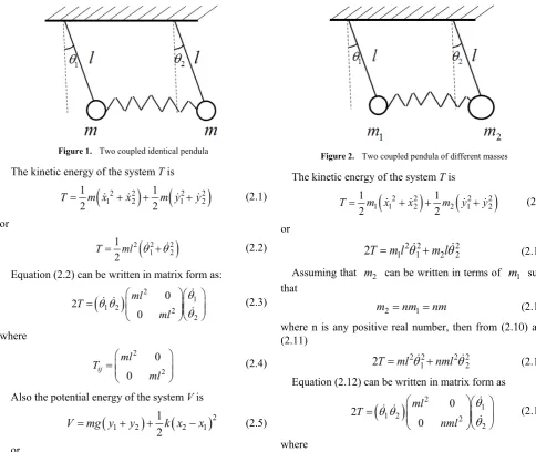
and length l _{coupled with a massless spring.} There is no kinetic energy associated with the motion of the spring with spring constant k (Fig. 1). The system has two degrees of freedom θ₁ and θ₂ which are the angles the rods make with the vertical [11].

Figure 1. Two coupled identical pendula The kinetic energy of the system T is

(

2 2

)

(

2 2

)

1 2 1 2

1 1

2 2

T = m x +x + m y +y (2.1) or

(

)

2 2 2 1 2

1 2

T= ml θ +θ (2.2) Equation (2.2) can be written in matrix form as:

(

)

2 1

1 2 ₂

2

0 2

0 ml T

ml θ θ θ

θ

  

= _  _{ }

 

 

  

 (2.3)

where

2

2

0 0

ij ml

T

ml

 

= _ _

 

(2.4)

Also the potential energy of the system V is

(

)

(

)

2

1 2 1₂ 2 1

V mg y= +y + k x −x (2.5) or

(

2

)(

2 2

)

2

1 2 1 2

1 ₂

2

V= _ mgl kl+ θ +θ − kl θ θ _ (2.6)

Equation (2.6) can be written in matrix form as

(

)

(

)

(

)

2 2

1

1 2 _{2 2}

2

2V mgl kl kl

kl mgl kl

θ θ θ

θ

 + −  

  

= _{  }

 − + _{ }

 

(2.7)

where

(

)

(

)

2 2

2 2

ij

mgl kl kl

V

kl mgl kl

 _{+ −} 

 

= _{ − +} _

 

(2.8)

2.1.2. Two Coupled Pendula of Different Masses

The system considered consist of two pendula of the same length l and different masses m₁ and m₂. The system has two degrees of freedom θ₁ and θ₂ which are the angles the rods make with vertical (Fig. 2).

Figure 2. Two coupled pendula of different masses The kinetic energy of the system T is

(

2 2

)

(

2 2

)

1 1 2 2 1 2

1 1

2 2

T= m x +x + m y +y (2.9) or

2 2 2 1 1 2 2

2

T m l

=

θ



+

m l

θ



(2.10) Assuming that m₂ can be written in terms of m₁ such that

2 1

m =nm nm= (2.11) where n is any positive real number, then from (2.10) and (2.11)

2 2 2 2

1 2

2T ml=

θ

 +nml

θ

 (2.12) Equation (2.12) can be written in matrix form as

( )

2 1

1 2 ₂

2

0 2

0 ml T

nml θ θ θ

θ

  

= _  _{ }

 

 

  

 (2.13)

2 2 0 0

ij ml

T

nml

 

= _ _

  (2.14)

also the potential energy of the system V is

(

)

2

1 1 2 2 1₂ 2 1

V m gy m gy= + + k x −x (2.15)

or

(

2

) (

2 2

)

2 2

1 2 1 2

2V= mgl kl+ θ + nmgl kl+ θ −2kl θ θ (2.16) and in matrix form

(

)

(

)

(

)

2 2 ₁

1 2 _{2 2}

2

2V mgl kl kl

kl nmgl kl

θ θ θ

θ  

 _{+ −} 

 

 

= _{  }

 − +  

  

(2.17)

where

(

)

(

)

2 2

2 2

ij

mgl kl kl

V

kl nmgl kl

 _{+ −} 

 

= _{ − +} _

 

(2.18)

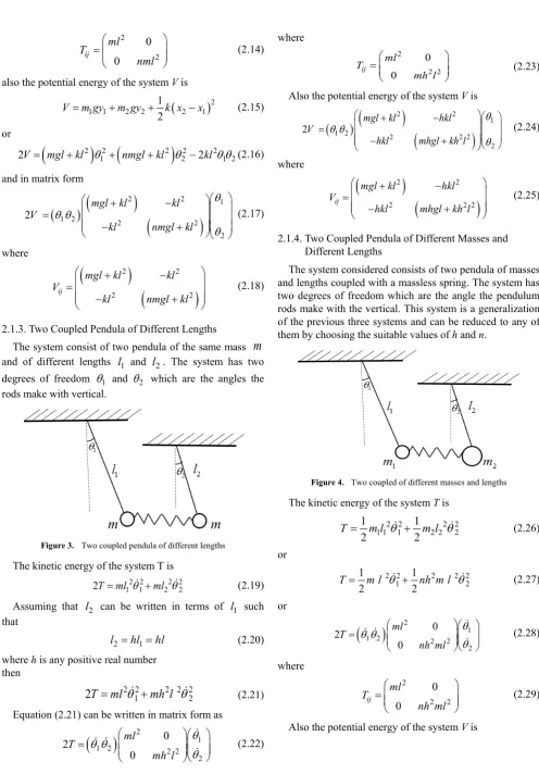
2.1.3. Two Coupled Pendula of Different Lengths

The system consist of two pendula of the same mass

m

and of different lengths l₁ and l₂. The system has two degrees of freedom θ₁ and θ₂ which are the angles the rods make with vertical.

Figure 3. Two coupled pendula of different lengths The kinetic energy of the system T is

2 2 2 2 1 1 2 2

2T ml= θ +ml θ (2.19) Assuming that l_{2 can be written in terms of} l₁ such that

2 1

l =hl =hl (2.20) where h is any positive real number

then

2 2 2 2 2

1 2

2

T ml

=

θ



+

mh l

θ



(2.21) Equation (2.21) can be written in matrix form as

(

)

2 1

1 2 _{2 2}

2 0 2

0 ml T

mh l θ θ θ

θ

  

= _  _{ }

 

 

  

 (2.22)

where

2

2 2

0 0

ij ml

T

mh l

 

= _ _

  (2.23)

Also the potential energy of the system V is

(

)

(

)

(

)

2 2

1

1 2 _{2 2 2}

2

2V mgl kl hkl

hkl mhgl kh l

θ θ θ

θ

 _{+ −  }

 _{ }

= _

 

 − + _{ }

 

(2.24)

where

(

)

(

)

2 2

2 2 2

ij

mgl kl hkl

V

hkl mhgl kh l

 _{+ −} 

 

= _{ − +} _

 

(2.25)

2.1.4. Two Coupled Pendula of Different Masses and Different Lengths

The system considered consists of two pendula of masses and lengths coupled with a massless spring. The system has two degrees of freedom which are the angle the pendulum rods make with the vertical. This system is a generalization of the previous three systems and can be reduced to any of them by choosing the suitable values of h and n.

Figure 4. Two coupled of different masses and lengths The kinetic energy of the system T is

2 2 2 2

1 1 1 2 2 2

1 1

2 2

T= m l θ + m l θ (2.26) or

2 2 2 2 2

1 2

1 1

2 2

T= m l θ + nh m l θ (2.27) or

( )

2 1

1 2 _{2 2}

2

0 2

0 ml T

nh ml θ θ θ

θ

  

= _  _{ }

 

 

  

 (2.28)

where

2

2 2

0 0

ij ml

T

nh ml

 

= _ _

  (2.29)

(

)

(

)

(

)

2 2

1

1 2 _{2 2 2}

2

2V mgl kl hkl

hkl nhmgl kh l θ θ θ

θ

 _{+ −  }

 _{ }

= _

 

 − + _{ }

 

(2.30)

where

(

)

(

)

2 2

2 2 2

ij

mgl kl hkl

V

hkl nhmgl kh l

 _{+ −} 

 

= _{ − +} _

 

(2.31)

2.2. Calculation of Power Flow of the System

The potential and kinetic energies are used to obtain the normal frequencies of the system using the secular equation

2 ₀

ij ij

V −

ω

T = (2.32) where

ω

is the natural frequency. Since all the four systems have two degrees of freedom, two values of

ω

are obtained in each case [11].

The normal modes of each system are obtained using the equation

2

₀

k k k

η



+

ω η

=

(2.33) where η is the normal co-ordinates and k =1,2 [11].

To convert the equations of motion from normal to generalized coordinates we use the equation

j jk k

k

a

θ

=

∑

η

(2.34)

Since for all the four systems k=1,2, we can write

1 11 12 1

21 22

2 2

a a

a a

θ

η

θ

η

    

=

    

 

    (2.35)

where

11 12 21 22

a a

a

a a

 

=  

  (2.36)

11

a and a21 are components of the eigenvector a1 which are computed by setting ω ω= ₁ and using [12]

11 2

1

21 0

ij ij a

V T

a

ω

 

 − _{ }=

 _{  } (2.37)

The same procedure applies for a12and a22which are components of eigenvector a2

The values of the a₁₁, a₂₁, a₁₂ and a₂₂ are obtained in terms of

m

and l using

†

ij

a T a I= (2.38) where a† is the Hermitian transpose of

a

_and I is the identity matrix. After obtaining the equations of motion in terms of generalized coordinates for each system, the effects

of damping and external forces is taken into consideration and the equations of motion are written in the form [13]:

( )

2

2

i i i i i i j

i i

F t

m m

εγ

θ

+

β θ

Ω + Ω

θ

= +

θ

(2.39)

where k=

εγ

, γ and

ε

are called the coupling parameters, Ω_i is the blocked frequency of the ith

oscillator and β_i is the damping ratio of the ith _oscillator.

The parameters from equation (2.39) are used to calculate the power flow. The first order approximation to the power flow between weakly coupled oscillators under white noise random excitations is given as

2 2

2 2 2 2

2( )

{( ) ( ) }{( ) ( )

ij

i i j j

oi

i j i i j j i j i i j j i j

U

m m p p p p

β β

ε γ

β β β β

=

 Ω + Ω 

 

Ω + Ω + − Ω + Ω + +

 

 

Π

(2.40)

where ₁ 2

i i i

p

= Ω −β and ₁ 2

j j j

p

= Ω −β

White noise is a random signal that is a combination of all audible frequencies (20Hz-20KHz) with constant power spectral density.

3. Results and Discussion

3.1. Identical Pendula System

Substituting equations (2.4) and (2.8) in equation (2.32) the natural frequencies of the system ω₁ and ω₂ are obtained as

1 g_l, 2 g_l 2_mk

ω = ω = + (3.1)

Substituting (3.1) in (2.33) gives

1 g_l 1 0

η

+ _{ }

η

=  

 (3.2)

2 g_l 2_mk 2 0

η

+_ + _

η

=

 

 (3.3)

Using equation (2.37) it can be shown that

2 2

11 21

0

kl a

kl a

−

+

=

and hence

11 21

a =a =α (3.4) Similarly,

2 2

21 22

0

kl a

kl a

−

−

=

and

21 22

a= α_{α −}β_β

  (3.6)

and using equation (2.38) we have

2

2

0 1 0

0 1 0

ml ml

α α α β

β β α β

 

    ₌ 

 

 ₋ _{ } ₋   

 _{ }   

or

2 2

2 2

2 0 1 0

0 1

0 2

m l

m l

α

β

 _{  }

=

 _{  }

 _{  }

 

(3.7)

and we obtain

11 21 1₂

a a

l m

= = (3.8)

and

21 22 1

2

a a

l m

= − = (3.9)

and hence equation (3.25) for this system is

1 1

2 2

2 2

2 2

1 1

2 2

1 1

2 2

ml ml

ml ml

θ η

θ η

 

   

 

   

 

 _{= }  



   

−

 

  _{ } 

    

(3.10)

From (3.10) we obtain the relationship between the normal coordinates and generalized coordinates for this system as

(

)

1 l m2 1 2

η

=

θ θ

+ (3.11) and

(

)

2 l m2 1 2

η

=

θ θ

− (3.12) If η₂=0 then θ₁=θ₂ and the two pendula oscillate in phase with an angular frequency ω₂= ( / ) (2 / )g l + k m and this is the first natural mode of the system. Also, if

1 0

η = then θ₁= −θ₂ and the two pendula oscillate in an out of phase mode with an angular frequency ω₁= g l/ and this is the second natural mode of the system [11].

The explicit equations of motion for this system are obtained by substituting (3.11) and (3.12) in (3.2) and (3.3) to give

(

θ θ 1+ 2

)

+g_l

(

θ θ1+ 2

)

=0 (3.13)

(

θ θ 1− 2

)

+_g_l +2_mk_

(

θ θ1− 2

)

=0 (3.14) By respectively adding and subtracting equations (3.13) and (3.14) and re-arranging we obtain

1 g k_{l m} 1 _mk 2 θ +_ + _θ = θ

 

 (3.15)

2 g k_{l m} 2 _mk 1

θ +_ + _θ = θ

 

 (3.16)

Multiplying equations (3.15) and (3.16) by the mass, m and adding the effects of damping and external forces we obtain

( )

1 1

1 c_m 1 g k_{l m} 1 F t_{m m}k 2

θ + θ +_ + _θ = + θ

 

  _(3.17)

( )

2 2

2 c_m 2 g k_{l m} 2 F t_{m m}k 1

θ + θ +_ + _θ = + θ

 

  _(3.18)

and comparing with (2.39) we can write (3.17) and (3.18) as

( )

1 2

1 2B1 1 1 F t_{m m}k 2

θ+ Ω + Ωθ θ = + θ (3.19)

( )

2 2

2 2B2 2 2 F t_{m m}k 1

θ + Ω + Ωθ θ = + θ (3.20)

where B1=_2mc1_Ω,B2=₂c_m2_Ω, F t1( )and F t2( )are two independent sources of stationary Gaussian white noise random excitation.

If F t₂( ) 0= , then equation (3.20) can be written as 2

2 2B2 2 2 _mk 1

θ

 + Ω + Ω

θ



θ

=

θ

(3.21)

and hence from equation (2.40), the rate of power flow from the first to the second pendulum can be written as

12 2 2

1 1 2

2 2 2 2 2

1 2 1 2 1 2 1 2

2( )

{( ) ( ) }{( ) ( )

o U

m p p p p

ε γ β β

β β β β

=

 Ω + Ω 

 

Ω + Ω + − Ω + Ω + +

 

 

Π

(3.22) The power input is dissipated by the damping of the second pendulum and hence the mean rate of power dissipation is

2 2

2 [ ] 22 2 [ ]2

c Eθ = mβ ΩEθ (3.23) Thus, equating equations (3.22) and (3.23) gives

2 2 2 2

1 1 2

2 2 2 2 2

2 1 2 1 2 1 2 1 2

1 2

( )

2 {( ) ( ) }{( ) ( )

2 2 [ ]

o

ml

l U

m p p p p

ε γ β β

β β β β β

θ

=

 Ω + Ω 

 

Ω  Ω + Ω + − Ω + Ω + + 



or

2 2 2 2

1 1 2

2 2 2 2 2

2 1 2 1 2 1 2 1 2

( )

2 o {( ) ( ) }{( ) ( )

T l U

m p p p p

ε γ β β

β β β β β

=

 Ω + Ω 

 

Ω _ Ω + Ω + − Ω + Ω + + _

(3.24) The blocked kinetic energy of the first pendulum is defined as the energy when the first oscillator is clamped so we can write

2 2

1B 1₂ml E[ ]o1 1₂Uo1

Substituting equation (3.25) in (3.24) we obtain

2 1

2 2 2

1 2

2 2 2 2 2

2 1 2 1 2 1 2 1 2

( )

{( ) ( ) }{( ) ( )

B T T

l

m p p p p

β β

ε γ

β β β β β

=

 Ω + Ω 

 

Ω Ω + Ω + − Ω + Ω + + 

(3.26) Equation (3.26) shows that the rate of power flow from the first pendulum to the second (when the latter is under white noise random excitations) is dependent on the blocked frequencies Ω₁, Ω₂and the damping coefficients

1

β , β₂. Since the blocked frequencies Ω₁and Ω₂are equal for this case, the rate of power flow will be maximum [13].

3.2. Two Coupled Pendula of Different Masses

Substituting equations (2.14) and (2.18) in (2.32) we obtain

(

)

(

)

2 4 4 2 2 3 4

2 2 2 3

2 1

1 0

nm l nm gl n mkl

nm g l n mgkl

ω −ω _ + + _

+ + + =

(3.27)

Solving equation (3.27) and retaining only positive frequencies (physically sound) we obtain the natural frequencies of the system ω₁and ω₂as

(

)

1 g_l, 2 g_l n_{n m}1 k

ω = ω = + + (3.28)

The system has two natural frequencies; the first is independent of the mass ratio and identical to that in section 3.1. The second natural frequency ω₂ is dependent on n and for large values of n, ω₂ tends to a constant value as

1 n+ →n.

The equations of motion are

1 g_l 1 0

η + _{ }η =  

 (3.29)

(

)

2 g_l n_{n m}1 k 2 0 η +_ + + _η =

 

 (3.30)

Since ω₁is the same as that of identical pendula, we can conclude that

11 21

a =a =α (3.31) Similarly, for ω₂ we obtain:

22 1 12

a a

n β

= − = (3.32)

Thus

1

a

n

α β

α β

 

 

= _{ −} _

 

(3.33)

and using (2.38) gives

2

2

0 0 0

1 1

0 0 0

ml

n nml n

α α α β

β β α β

  _{ }

 _{ } 

 

 _{ } _{ =}

 

 ₋   ₋ 

     

 _{ }   

(3.34)

Solving equation (3.34), the values of

α

and

β

are obtained as

(

11

)

l n m

α=

+ (3.35)

and

(

)

1 1 /

l m n n

β =

+ (3.36)

Thus

(

)

(

)

(

)

(

)

1

1

2 2

1 1

1 1 /

1

1 1 /

l n m l m n n

n

l n m l m n n

η θ

θ η

  

  _

 

  _{+ +}

  

  =   

  _ −

 

  _{  }

+ +

    

(3.37)

Equation (3.37) gives

(

)

(

)

1 1 1 1 2

1 1 /

l n m l m n n

θ = η + η

+ + (3.38)

and

(

)

(

)

2 1 1 1 2

1 1 /

l n m l m n n

θ = η − η

+ + (3.39)

Using (3.38) and (3.39) the equations of motion are obtained as

(

nθ θ 1+ 2

)

+ g_l

(

nθ θ1+ 2

)

=0 (3.40)

(

θ θ1 2

)

g_l

(

n_{n m}1

)

k

(

θ θ1 2

)

0

 + 

− +_ + _ − =

 

  (3.41)

Adding equations (3.40) and (3.41) and re-arranging we obtain

(

)

1 2 1

2

( 1) ( 1)

2 2

1 ( 1)

2 2

n g n k

l n m

n g n k

l n m

θ θ θ

θ

−  + 

+ +_ + _

 

 − + 

=_ + _

 

 

(3.42)

Assuming that

θ



₂ can be written in terms of

θ



₁ as

2

s

1

θ



=

θ



, where s is any positive real number and taking

mg d

kl

= , then (3.42) becomes

1 c1 1_{p l}g ( 1)n_{2n m}k 1 1 (1 )_p n n d n_2n ( 1) _mk 2

θ + θ+ _ + + _θ = _ − + + _ θ

   

  (3.43)

where 2

2 sn s p= − +

2 g_l 1_{n m}k 2 1_{n m}k 1

θ +_ + _θ = θ

 

 (3.44)

Multiplying equation (3.43) and (3.44) by the respective masses, adding the damping and the external force terms gives

1

1 1 1

1 1

2

1 2

1 ( 1)

2 ( ) 1 (1 ) ( 1)

2

c g n k

m p l n m

F t n n d n k

m p n m

θ θ θ

θ

+

 

+ + _ + _

 

− + +

 

= _{+  }

 

 

(3.45)

( )

2 2

2 2 2 1

2 2 1

1 F t

c g k k

m l n m m m

θ + θ +_ + _θ = + θ

 

  (3.46)

Equations (3.45) and (3.46) can be re-written as

( )

1 2

1 1 1 1 1 1 2

1 1

(1 ) ( 1)

2

2

F t n n d n

B

m n m

εγ

θ + Ωθ + Ωθ = _{+ } − + + _ θ

 

 

(3.47)

( )

2 2

2 2 2 2 2 2 1

2 1

2B F t

m m

εγ

θ + Ωθ + Ωθ = + θ (3.48)

where 1

1 1 1 2

c B

m =

Ω , 2 2 _{2 2}2

c B

m =

Ω , Ω =12 1_{p l}_g+( 1)a₂+_{a m}k_

 ,

2

2 g_{l a m}1 k

Ω = +

Setting F t₂( ) 0= , then the rate of power flow from the first to the second pendulum can be written as

{

}{

}

12 2 2

1 1 1 2 2

2 2 2 2

1 2 _{1 1 2 2 1 2 1 1 2 2 1 2}

2( )

( ) ( ) ( ) ( )

o

U f

m m _{p p p p}

ε γ β β

β β β β

=

 _{Ω + Ω} 

 

 _{Ω + Ω + − Ω + Ω + +} 

 

Π

(3.49)

where (1 ) ( 1)

2

n n d n f

n

− + +

 

= _ _

Thus, since the power input is dissipated by the damping of the second pendulum, the mean rate of power dissipation can be equated to (3.49) giving

{

}{

}

2 2 2 2

1 1 1 2 2

2 2 2 2

1 2 2 1 1 2 2 1 2 1 1 2 2 1 2

( )

2 ( ) ( ) ( ) ( )

o

T

l U f

m m p p p p

ε γ β β

β β β β β

=

 _{Ω + Ω} 

 

 

Ω_ Ω + Ω + − Ω + Ω + + _

(3.50) The blocked kinetic energy of the first pendulum 1

T

B is related to (3.50) as

2 1

2 1 1 2 2 2 2 1

2 2 2 2

2 2 1 2 2 2 1 2

1 1

1 1 1 1

1 B

T T

C

p p p p

β β

β β

β β

=

 

 ₊ Ω  Ω

 

 _{Ω Ω }

  

_{ Ω   − } _{ Ω   − } 

 _{+ +}  _{+ +} 

 _Ω   _Ω   _Ω   _Ω  

       

  

  

(3.51)

where 2 2 2_{2 2}

1 2 1 2

l f C

m m

ε γ

=

Ω Ω is the coupling parameter and the

greater the value of Cthe stronger the coupling. For weak coupling, _C=10−4 _and

1 2 0.01

β =β = . Thus equation (3.60) can be plotted using the calculated parameters in Table 3.1 as in Fig. 3.1.

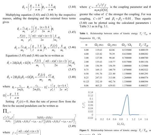
Table 1. Relationship between ratios of kinetic energy T T₂ / _1B and frequencies Ω₂ /Ω₁

H Ω₁(Hz) Ω₂(Hz) Ω₂/Ω₁ T T₂/ _1B 6.00 119.63 64.06 0.535000 0.000159 4.00 123.82 78.39 0.633000 0.000282 3.00 127.88 90.48 0.708000 0.000780 2.00 135.63 110.77 0.817000 0.001156 1.00 156.59 156.59 1.000000 0.125000 0.75 169.13 180.79 1.070000 0.002522 0.50 191.76 221.40 1.150000 0.001295 0.25 247.53 313.08 1.260000 0.000574 0.125 332.10 442.74 1.330000 0.000394 0.06 465.23 639.03 1.370000 0.000327

Figure 5. Relationship between ratios of kinetic energy T T₂ / _1B and frequencies Ω₂/Ω₁

Equation (3.51) shows the rate of power flow from the first to the second pendulum. Fig. 5 is a plot of the kinetic energy of the second pendulum T2 to the blocked energy of

the first T1B against the ratios of blocked frequency

2/ 1

Ω Ω . Fig.3.1 shows that T2/ T1B is maximum when

2/ 1

Ω Ω equals one and is minimum when it tends to zero or infinity [13].

3.3. Two Coupled Pendula of Different Lengths

Equation (2.32) for this system gives

(

)

(

)

2 2 4 4 2 2 4 2 3

2 2 2 3

2 1

1 0

h m l h mkl h h m gl

hm g l h h mgkl

ω −ω _ + + _

+ + + = (3.52)

If we let _{ω =}4 _x2 _then

(

)

(

)

2 2

2 2 2

1 ₁ 1

2 4

h h g

k g k

x

m h l m h k l

+ −

= + ± + (3.53)

-0.020 0.02 0.04 0.06 0.08 0.1 0.12 0.14

0 0.2 0.4 0.6 0.8 1 1.2 1.4 1.6

T1 /T2

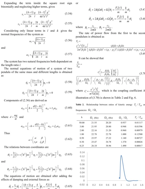
Expanding the term inside the square root sign binomially and neglecting higher terms, gives

(

)

(

)

2 2

1 2 2 2

1 1

2 4

h g h g

x

h l h k l

+ −

= − (3.54)

(

)

(

)

2 2

2 2 2 2

1 2 1

2 4

h g k h g

x

h l m h k l

+ −

= + + (3.55)

Considering only linear terms in l and k _{gives the} normal frequencies of the system as

( )

1 h_{2h l}1 g

ω = + (3.56)

and

(

)

2 h_{2h l}1 g 2_mk

ω = + + (3.57)

The system has two natural frequencies both dependent on the length ratio l.

The normal equations of motion of a system of two pendula of the same mass and different lengths is obtained as

(

)

1 h_{2h l}1 g 1 0

η + + η =

 

 (3.58)

(

)

2 h_{2h l}1 g 2_mk 2 0

η +_ + + _η =

 

 (3.59)

Components of (2.36) are derived as

1

21 d(1 )₂ h 11 2 11

a =_h+ − _− a =τ a

  (3.60)

where d mg kl = _and

1

22 d(1₂ h) 12 2 12

a = − +_ h − _− a =ξ a

  (3.61)

Thus

1 2 a_{= }_{τ α ξ β}α β 

  (3.62)

The relations between coordinates are

(

2 2

)

12

(

2 2

)

12

1 1_l 1 ih m 1 1_l 1 ih m 2 θ ₌  ₊τ − η ₊  ₊ξ − η

    (3.63)

and

(

2 2

)

12

(

2 2

)

12

2 τ_li 1 ih m 1 ξ_li 1 ih m 2 θ ₌  ₊τ − η ₊  ₊ξ − η

    (3.64)

The equations of motion are obtained after adding the effects of damping and external forces as

( )

1 1

1 c_m 1 (h_{2h l m}1)g k 1 F t_{m m}k 2 θ + θ +_ + + _θ = + θ

 

  (3.65)

( )

2 2

2 2 ( ₂1) 2 1

2

F t

c h g k k

m h l m m m

θ + θ +_ + + _θ = + θ

 

  (3.66)

or

( )

1 2

1 2B1 1 1 1 F t_{m m}k 2

θ+ Ω + Ωθ θ = + θ (3.67)

( )

2 2

2 2B2 2 2 2 F t_{m m}k 1

θ + Ω + Ωθ θ = + θ (3.68)

where 1

1 ₂c

B m =

Ω, 2 2 2

c B

m =

Ω.

The rate of power flow from the first to the second pendulum is obtained as

2 2 2 2

2 1 1 2

2 2 2 2 2

2 1 2 1 2 1 2 1 2

( )

2 {( ) ( ) }{( ) ( )

o T

l U

m p p p p

ε γ β β

β β β β β

=

 Ω + Ω 

 

Ω  Ω + Ω + − Ω + Ω + + 

(3.69) It can be showed that

2 1

2 1 1 2 2 2 2 1

2 2 2 2

2 2 1 2 2 2 1 2

1 1

1 1 1 1

1 B

T T

C

p p p p

β β

β β

β β

=

 

 ₊ Ω  Ω

 

 _{Ω  }

Ω

  

_{ Ω   − } _{ Ω   − } 

 _{+ +}  _{+ +} 

 _Ω   _Ω   _Ω   _Ω  

       

  

  

(3.70)

where 2 2 22 2 2 2

1 2

l C

m

ε γ

=

Ω Ω which is the coupling coefficient An

illustration of (3.70) is shown in Table 2 and Fig. 6.

Table 2. Relationship between ratios of kinetic energy T T₂ / _1B and frequencies Ω₂ /Ω₁

h Ω₁(Hz) Ω₂(Hz) Ω₂ /Ω₁ T T2/ 1B 50.00 21.55 20.20 0.937 0.01117

3.00 21.95 20.80 0.948 0.01596 2.00 22.16 21.20 0.960 0.00979 1.00 22.78 22.78 1.000 0.12500 0.50 23.97 27.22 1.140 0.00727 0.30 25.47 34.78 1.370 0.00026 0.25 26.18 38.96 1.490 0.00017

Figure 6. Relationship between ratios of kinetic energy T T₂/ _1B and frequencies Ω₂ /Ω₁

-0.02 0 0.02 0.04 0.06 0.08 0.1 0.12 0.14

It is observed from Fig. 6 that the power flow is maximum when the ratio of blocked frequencies is 1.

3.4. Compound Pendula with Different Masses and Lengths

Here, equation (2.32) gives

(

)

(

)

2 2 4 4 2 2 4 2 3

2 2 2 3

( 1) 1

0

nh m l n h mkl nh h m gl

nhm g l h h n mgkl

ω −ω _ + + + _

+ + + =

(3.71)

Considering only terms that are linear in lwe can write the natural frequencies ω₁ and ω₂ of the system as

1 _{h n}(₍n h g₁₎) _l

ω = +

+ (3.72)

(

)

2 _{h n}nh₍ 1₁₎g_l (n_nm1)k

ω = + + +

+ (3.73)

Thus, the normal equations of motion are

(

)

1 _{h n(}h n g_{1) l} 1 0

η + + η =

+

 (3.74)

(

)

2 _{h n}nh₍ 1₁₎g_l (n_nm1)k 2 0 η +_ + + + _η =

+

 

 (3.75)

Also,

1 2

21 dn h a₍( ₁₎ ) 11 2 11

a h a a

n τ

−

 ₋ 

=_ + _ =

+

  (3.76)

1

22 dn h₍( ₁₎1) 12 2 12

a nh a a

h n ξ

−

 − 

= − +_{ } =

+

  (3.77)

and

a= _{τα ξβ}α β 

  (3.78)

Hence

(

)

(

)

(

)

(

)

1 1

2 2 2 2 2 2

1

1 1

2 2 2 2 2 2

1

1 ₁ 1 ₁

1 1

h m h m

l l

a

h m h m

l l τ ξ τ _τ ξ _ξ − − − −        _ + _{ } + _    =     ₊   ₊    _{   }    (3.79) and

(

)

(

)

1 2 2 2

1 2 1 1

1 2 2 2

2 (1 _{) 1} (1 _{) 1}

h m l h m l τ θ θ τ η ξ _{ξ η} − − +   + = _ + _ + _{ } + _ + _ (3.80)

(

)

(

)

1 2 2 2

1 2 1 1

1 2 2 2

2

(1 _{) 1}

(1 _{) 1}

h m l h m l τ θ θ τ η ξ _{ξ η} − − −   − = _ + _ − _{ } + _ + _ (3.81)

Assuming that η₂ =qη_{1 where q is any real number, we} can re-write equations (3.80) and (3.81) as

(

)

1 2 1 2

( ) ( ) 0

( 1) h n g

h n l

θ θ+ +_ + _θ θ+ = +

 

  (3.82)

(

)

1 2 1 ( 1) 1 2

( ) ( ) 0

( 1)

nh g n k

h n l n m

θ θ− +_ + + + _θ θ− = +

 

  (3.83)

The equations of motion are obtained as:

( )

1

1 1 1

1 1 1

1

2

1 1

( 1) ( 1) ( 1)

2 ( 1) 2

c h n h g n k

m h n l n m

F t _f k

m m θ θ θ θ  + + + +  + +_ + _ +   = +   (3.84)

( )

2

2 2 2

2 2 2

2

1

2 2

( 1) ( 1) ( 1)

2 ( 1) 2

c h n h g n k

m h n l n m

F t _f k

m m θ θ θ θ  + + + +  + +_ + _ +   = +   (3.85) or

( )

1 2

1 1 1 1 1 1 2

1 1

2B F t f k

m m

θ+ Ωθ + Ω θ = + θ (3.86)

( )

2 2

2 2 2 2 2 2 1

2 2

2B F t f k

m m

θ + Ωθ + Ωθ = + θ (3.87)

Where 1

1 1 1 2 c B m =

Ω , 2 2 _{2 2}2 c B

m

=

Ω and

( 1)( 1) ( 1)

( 1) 2

d n h n f

h n n

− − +

= +

+

The rate of power flow from the first to the second pendulum is

{

}{

}

2 2 2 2

2 1 1 1 2 2

2 2 2 2 2

2 2 1 1 2 2 1 2 1 1 2 2 1 2

( )

2 ( ) ( ) ( ) ( )

o

T

l U

nm p p p p

ε γ β β β β β β β =  _{Ω + Ω}      Ω _ Ω + Ω + − Ω + Ω + + _ (3.89) and the blocked kinetic energy T_1B of the first pendulum is related to the power flow as:

2 1

2 1 1 2 2 2 2 1

2 2 2 2

2 2 1 2 2 2 1 2

1 1

1 1 1 1

1 B

T T

C

p p p p

β β β β β β =    ₊ Ω  Ω    _{Ω Ω }    _{ Ω   − } _{ Ω   − }   _{+ +}  _{+ +}   _Ω   _Ω   _Ω   _Ω                 (3.90)

where 2 2 22 1 2 2 2 2 o l U C nm ε γ β = Ω

Equation (3.90) can be illustrated as in Table 3 and Fig. 7.

Equation (3.90) shows the rate of power flow from the first to the second pendulum when the first is under white noise random excitations and Fig. 7, is a plot of T2/ T1B

Table 3. Relationship between ratios of kinetic energy T T₂/ ₁B and

frequencies Ω₂/Ω₁

N H Ω1

(Hz) 2 Ω

(Hz) Ω Ω2/ 1 T T2/ 1B 4.00 4.00 123.79 61.90 0.500000 0.000133 3.00 3.00 127.85 73.45 0.570000 0.000444 2.00 2.00 135.67 95.89 0.710000 0.000588 1.00 1.00 156.59 156.59 1.000000 0.124900 0.90 0.90 160.84 169.74 1.055000 0.014820 0.80 0.80 166.08 185.61 1.120000 0.003530 0.70 0.70 172.25 206.26 1.200000 0.001347 0.60 0.60 180.93 232.26 1.280000 0.000709 0.50 0.50 191.78 271.22 1.410000 0.000347

Figure 7. Relationship between ratios of kinetic energy T T_{2/ 1B} and frequencies Ω₂/Ω₁

3.5. Application of Power Flow in Compound Pendulum to an Optical Switch

Fig. 8 shows an optical switch which is a device that allows optical signals to be switched on and off or switched from one channel to another. An optical switch is made of two parallel waveguides coupled with a directional coupler [14]. A directional coupler is made of two optical waveguides that are brought close to each other in such a way that their respective optical modes can interact and split into even and odd symmetries that allow the transfer of power between them [15]. For an optical switch, the relative phase difference between the supermodes of the coupling

system must be π and hence the value of the coupling length

Lc must be chosen to satisfy this condition.

Figure 8. A schematic diagram of an optical switch [16] Fig. 9 explains the theory of switching in an optical directional coupler, in Fig. 9 (a) the optical signal is

transferred through the upper waveguide, at z=0, the two modes interact, the odd mode is shown with red while the even mode is blue. The region where both symmetries interfere (shown in green in (Fig. 9 (b))) is where is optical signal is transmitted to. Similarly at z L= _c, the phase shift

between the even mode and odd mode is π and the

interaction between the two mode leads to the switching of the optical signal from the upper to the lower waveguide (Fig. 9 (c) and (d)).

(a)

(b)

(c)

(d)

Figure 9. Theory of switching [16]

Coupled pendulum system is analogous to coupled transmission lines and understanding the behavior of coupled pendulum system can aid in explaining the behavior of coupled transmission lines and other related devices. In 1996, the coupled mode theory was used to analyze both systems and it was found that a system of two weakly coupled identical pendula and two weakly coupled

-0.02 0 0.02 0.04 0.06 0.08 0.1 0.12 0.14

0 0.2 0.4 0.6 0.8 1 1.2 1.4 1.6

T2 /T1

pendula of different lengths can be used to model the basic behavior of an optical switch. In an optical switch, a deriving voltage is used to change the phase constants of the waveguides, when the phases are equal, the power is transferred between the waveguides and when the voltage is applied, the phase constants are no longer equal and there is no power transfer between the waveguides [17].

From Fig 9, it can be deduced that the effect of the driving voltage can be visualized as changing the length ratio of the pendula system and the net power flow corresponds to the case when h=1 i.e. when the system reduces to the identical pendula case. When h≠1, the phase constants are not equal and hence there will be no net power flow between the waveguides.

4. Conclusions

The coupled pendula system has been used for decades as a model to simulate natural phenomena and hence knowing the natural and blocked frequencies, general equations of motion and rate of power flow between the components of such systems is crucial. In this research work, four cases of two weakly coupled pendula systems were taken into consideration. Analytical tools were used to derive the rate of power flow under white noise random excitations between the two oscillators. Higher order terms of the frequencies can be included to obtain more accurate results. Future researches may be done to obtain the same parameters for strongly coupled pendula. Computational and experimental components can be added to this research.

REFERENCES

[1] Serway, R. A. and Jewett, J.W. Physics for scientists and engineers, with modern physics. Belmont, CA, Thomson-Brooks/Cole, 2003, 452-485.

[2] Ndikilar C.E. and Maharaz M. N. Elementary Space Science, ABU Press, Zaria, 2016.

[3] Strogatz, S.H. and Stewart, I. A subtle mathematical thread connects clocks, ambling elephants, rhythms and onset chaos. Scientific American Journal, 1993, 269(6): 102-107.

[4] Schubert, K. R. and Stiewe, J. (2011). Demonstration of K0K0, B0B0 and D0D0 Transitions with a Pair of Coupled Pendula. Journal of Physics G: Nuclear and Particle Physics, 2011, 39(3), 33-110.

[5] Singiresu, S. R. (2011). Mechanical vibrations. Prentice Hall, 1 Lake Street, Upper Saddle River, 2011, 210-323.

[6] Mallada, E. and Tang, A. Synchronization of weakly coupled oscillators: coupling. Journal of Physics, 2013, 46(50): 501-510.

[7] Yaniv, Y.. Lakatta, E. G. and Maltsev, V. A. From two competing oscillators to one coupled-clock pace maker cell system. Frontiers in Physiology Journal, 2015, 48(12): 667-684.

[8] Ramana, R. A, Sen, A. and Johnston. G.L. Experimental evidence of time-delay-induced death in coupled limit-cycle oscillators. Physical Review Letters, 2000, 85 (16): 3381-3384.

[9] Kubacki, M. Dynamics of Coupled Double Pendulums, 2011, [online] Avalable: (April 7, 2018).

[10] Altshulera E. and Garcia, R. Josephson junctions in a magnetic field: Insights from coupled pendula. American Journal of Physics, 2003, 71(4): 405-408.

[11] Ndikilar, C. E.. Analytical Mechanics, ABU Press, Zaria, 2018, (In press).

[12] Shapiro, J.A. Classical mechanics. Rutgers university, University press New Jersey, United States of America, 2003, 1-35.

[13] Newland, D. E. Calculation of power flow between coupled oscillators. Journal of Sound and Vibration, 1966, 3(3): 262-276.

[14] Vakili, B. Bahadori, S.and Ghayour, R. All-optical switching using a new photonic crystal directional coupler. Advanced Electromagnetics,2015, 4:63-67.

[15] Beggs, D. M. White, T. P. O’Faolain, L. and Krauss, T. F. Design and fabrication of a photonic crystal directional coupler for use as an optical switch. 2008, 379-382.

[16] Yamada, H. Chu, T. Ishida, S. and Arakawa, Y. Optical directional coupler based on Si-wire waveguides. IEEE photonic technology letters, 2005, 17(3): 585-588.