SCHEDULING IN DISTRIBUTED SYSTEMS: A SURVEY AND FUTURE PERSPECIVE

152 |

P a g e

SCHEDULING IN DISTRIBUTED SYSTEMS:

A SURVEY AND FUTURE PERSPECIVE

Reeta Koshy

Assistant Professor, Sardar Patel Institute of Technology, Mumbai (India)

ABSTRACT

In a distributed system it can occur that some nodes are idle or lightly loaded while others are heavily loaded.

This leads to the opportunity of improving the performance of a distributed system as a whole by remote

execution and migrating jobs from heavily-loaded nodes to idle or lightly-loaded nodes. It is the task of the

distributed scheduler to schedule processes to nodes (processors) in some optimal way. Distributed scheduling is

an NP complete problem. We discuss the early scheduling paradigms. Bee Colony optimization is an algorithm

in swarm intelligence category. This algorithm is based on the intelligent behavior of honey bees in foraging

process

Keywords:

I INTRODUCTION

The main objective of scheduling is to enhance system performance metrics such as process completion time and

processor utilization. Scheduling processes onto processors is challenging due to the presence of multiple

processing nodes.

1.1 Properties of a Good Scheduler

A good scheduling approach s h o u l d support heterogeneous resources, placement objective function(s),

scalability, co scheduling methods, and assumptions about system configuration. A good scheduler should have

the following properties:

General purpose: A scheduling approach should make few assumptions and have few restrictions to the types

of applications that can be executed. Different kinds of jobs, distributed and parallel applications, interactive

jobs, as well as non-interactive batch jobs, should all be supported with good performance. This property is

difficult to achieve. Because different kinds of jobs have different attributes, their requirements to the

scheduler may contradict. To achieve this general purpose, a tradeoff may have to be made.

Efficiency: First it should improve the performance of scheduled jobs as much as possible; second is that the

scheduling should incur reasonably low overhead.

Fairness: user obtains his/her fair share when demand is heavy.

Dynamic: the algorithms employed to decide where to process a task should respond to load changes, and

153 |

P a g e

Transparency: the result of a task’s execution should not be affected by local and remote execution. No user

effort should be required in deciding where to execute a task or in initiating remote execution.

Local scheduling: where each workstation independently schedules its processes, is easy to construct, scalable,

fault-tolerant, etc. Meanwhile, coordinated scheduling of parallel jobs across the nodes of a multiprocessor (co

scheduling) is also an option in a distributed system..

II EARLY SCHEDULING PARDIGMS

Several scheduling paradigms emerge, depending on

a) Whether a system performs schedulability analysis,

b) If it does, whether it is done statically or dynamically, and

c) Whether the result of the analysis itself produces a schedule or plan according to which tasks are dispatched at

run-time.

Based on this we can identify the following classes of algorithms:

2.1 Static Table-Driven Scheduling

Resources needed to meet the deadlines of safety-critical tasks must be preallocated so that they can be

guaranteed a priori. These tasks are usually statically scheduled such that their deadlines will be met even under

worst case conditions. These tasks are assumed to be periodic. For periodic tasks,there exists a feasible schedule

if and only if there exists a feasible schedule for the LCM (the least common multiple) of the periods. Given a set

of periodic tasks, a typical algorithm that deals with multiprocessors or a distributed system attempts to assign

subtasks to sites in the system and construct a schedule of length LCM of the the task periods. At run time, the

set of tasks is repeatedly executed according to this schedule every LCM units of time. If the tasks have simple

characteristics, then a table can be constructed using the earliest-deadline-first (EDF), or the shortest-period-first

technique.

2.2 Priority-Driven Preemptive Scheduling

Priority- driven preemptive scheduling is used in most time-sharing systems. In non-real-time systems, the

priority of a job changes depending on whether it is CPU-bound or I/O-bound. In real-time systems, priority

assignment is related to the time constraints associated with a job or task and this assignment can be either static

or dynamic. There are two preemptive algorithms. The first algorithm, called the Rate-Monotonic (RM)

algorithm assigns static priorities to tasks based on their periods. It assigns higher priorities to tasks with shorter

periods. Second, Earliest-Deadline-First (EDF), a dynamic priority-assignment algorithm: The closer a task’s

deadline, the higher its priority.

In static priority a task’s priority is assigned once it arrives and is not reevaluated as time progresses. The RM

priority-assignment policy is applicable to periodic tasks. A dynamic priority assignment policy, however, can be

154 |

P a g e

expensive in terms of run-time overheads.

2.3 Dynamic Planning-Based Scheduling

In dynamic planning-based schedulers, dynamic feasibility checks are performed. A task is guaranteed by

constructing a plan for task execution whereby all guaranteed tasks meet their timing constraints. A task is

guaranteed subject to a set of assumptions, for example, about its worst case execution time and resource needs,

and the nature of faults in the system. If these assumptions hold, once a task is guaranteed it will meet its timing

requirements. A guarantee algorithm must consider many issues including worst case execution times, resource

requirements, timing constraints, the presence of periodic tasks, preemptable tasks, precedence constraints

(which is used to handle task groups), multiple importance levels for tasks, and fault- tolerance requirements. In

a distributed system, when a task arrives at a site, the scheduler at that site attempts to guarantee that the task will

complete execution before its deadline, on that site. If the attempt fails, the scheduling components on individual

sites cooperate to determine which other site in the system has sufficient resource surplus to guarantee the task.

With regard to cooperation between processing elements, several schemes exist. In the random scheduling

algorithm, the task is sent to a randomly selected site; in the focussed-addressing algorithm, the task is sent to a

site that is estimated to have sufficient surplus resources and time to complete the task before its deadline; in the

bidding algorithm, the task is sent to a site based on the bids received for the task from sites in the system; and in

the flexible algorithm, the task is sent to a site based on a technique that combines bidding and focused

addressing.

2.4 Dynamic Best Effort Scheduling

Best effort scheduling is the approach used by many real-time systems deployed today. In such systems, a

priority value is computed for each task based on the task’s characteristics and the system schedules tasks

according to their priority. Confidence is gained in the system via extensive simulations, in conjunction with

recoding the tasks and priority adjustment. Clearly, the biggest disadvantage of dynamic best effort algorithms

lies in their lack of predictability and their sub optimality. A dynamic scheduling algorithm is said to be optimal

if it always produces a feasible schedule whenever a clairvoyant algorithm, i.e., a static scheduling algorithm

with complete prior knowledge of the tasks, can do so.

III Local Scheduling

In a distributed system, local scheduling means how an individual workstation should schedule those processes

assigned to it in order to maximize the overall performance. In a distributed system, the local scheduler may need

global information from other workstations to achieve the optimal overall performance of the entire system.

Here, we introduce two scheduling techniques One is a proportional-sharing scheduling approach, in which the

resource consumption rights of each active process are proportional to the relative shares that it is allocated.

Second is predictive scheduling, which is adaptive to the CPU load and resource distribution of the distributed

155 |

P a g e

.1 Proportional-Sharing Schedule

With proportional-share scheduling, the resource consumption rights of each active process are proportional to

the relative shares that it is allocated. Stride scheduling is an example of proportional-sharing schedule fairly

allocating a single processor among competing users on a single-node.

In section 4.1.2, two extensions of stride scheduling are presented to provide better response-times for interactive

jobs. Finally, fairness can also be guaranteed when stride scheduling is used in a distributed cluster.

3.1.1 Stride Scheduling

As a kind of proportional-share scheduling strategies, stride scheduling allocates resources to competing users in

proportion to the number of tickets they hold. Each user has a time interval, or stride, inversely proportional to

his/her ticket allocation, which determines how frequently it is used. A pass is associated with each user. The

user with a minimum pass is scheduled at each interval; a pass is then incremented by the job's stride. Figure 1 is

an example of stride scheduling.

Figure 1.Stride Scheduling

3.1.2 Extensions to Stride Scheduling

In order to handle the interactive and I/O intensive job workloads, stride scheduling must be extended to improve

the responsive time and I/O throughput, while not penalizing competing users. Jobs are given incentive to

relinquish the processor when not in use and will receive their share of resources over a longer time-interval.

Thus, because interactive jobs are scheduled more frequently when they awaken, they can receive better response

time. The first approach is loan & borrow, and the second approach is system credit. Both approaches are built

upon exhaustible tickets, which are simple tickets with expiration time.

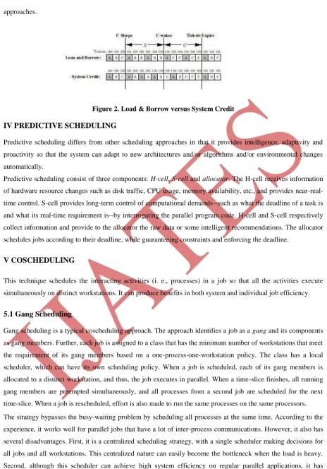
Loan & Borrow: In this approach, when a user temporarily exits the system, other users can borrow these

otherwise inactive tickets. The borrowed tickets expire when the user rejoins the system. When the sleeping user

wakes up, it stops loaning tickets and is paid back in exhaustible tickets by the borrowing users. In general, the

lifetime of the exhaustible tickets is equal to the length the original tickets were borrowed. This policy can keep

the total number of tickets in the system constant over time; thus, users can accurately determine the amount of

resources they receive.

System Credit: This second approach shown in Figure 2 is an approximation of the first one. With system

credits, clients are given exhaustible tickets from the system when they awaken. The idea behind this policy is

that after a client sleeps and awakens, the scheduler calculates the number of exhaustible tickets for the clients to

receive its proportional share over some longer interval. The system credit policy is easy to implement and does

156 |

P a g e

Figure 2. Load & Borrow versus System Credit

IV PREDICTIVE SCHEDULING

Predictive scheduling differs from other scheduling approaches in that it provides intelligence, adaptivity and

proactivity so that the system can adapt to new architectures and/or algorithms and/or environmental changes

automatically.

Predictive scheduling consist of three components: H-cell, S-cell and allocator. The H-cell receives information

of hardware resource changes such as disk traffic, CPU usage, memory availability, etc., and provides

near-real-time control. S-cell provides long-term control of computational demands--such as what the deadline of a task is

and what its real-time requirement is--by interrogating the parallel program code. H-cell and S-cell respectively

collect information and provide to the allocator the raw data or some intelligent recommendations. The allocator

schedules jobs according to their deadline, while guaranteeing constraints and enforcing the deadline.

V COSCHEDULING

This technique schedules the interacting activities (i. e., processes) in a job so that all the activities execute

simultaneously on distinct workstations. It can produce benefits in both system and individual job efficiency.

5.1 Gang Scheduling

Gang scheduling is a typical coscheduling approach. The approach identifies a job as a gang and its components

as gang members. Further, each job is assigned to a class that has the minimum number of workstations that meet

the requirement of its gang members based on a one-process-one-workstation policy. The class has a local

scheduler, which can have its own scheduling policy. When a job is scheduled, each of its gang members is

allocated to a distinct workstation, and thus, the job executes in parallel. When a time-slice finishes, all running

gang members are preempted simultaneously, and all processes from a second job are scheduled for the next

time-slice. When a job is rescheduled, effort is also made to run the same processes on the same processors.

The strategy bypasses the busy-waiting problem by scheduling all processes at the same time. According to the

experience, it works well for parallel jobs that have a lot of inter-process communications. However, it also has

several disadvantages. First, it is a centralized scheduling strategy, with a single scheduler making decisions for

all jobs and all workstations. This centralized nature can easily become the bottleneck when the load is heavy.

Second, although this scheduler can achieve high system efficiency on regular parallel applications, it has

157 |

P a g e

interactive response, making them a less attractive choice for use in a distributed system. These limitations

motivate the integrated approaches.

5.2 Implicit Coscheduling

Implicit coscheduling is a distributed algorithm for time-sharing communicating processes in a cluster of

workstations. By observing and reacting to implicit information, local schedulers in the system make

independent decisions that dynamically coordinate the scheduling of communicating processes. The principal

mechanism involved is two-phase spin-blocking: a process waiting for a message response spins for some

amount of time, and then relinquishes the processor if the response does not arrive.

The spin time before a process relinquishes the processor at each communication event consists of three

components. First, a process should spin for the baseline time for the communication operation to complete; this

component keeps coordinated jobs in synchrony. Second, the process should increase the spin time according to

a local cost-benefit analysis of spinning versus blocking. Third, the pairwise cost-benefit, i.e., the process, should

spin longer when receiving messages from other processes, thus considering the impact of this process on others

in the parallel job.

 The baseline time comprises the round-trip time of the network, the overhead of sending and receiving

messages, and the time to awake the destination process when the request arrives.

 The local cost-benefit is the point at which the expected benefit of relinquishing the processor exceeds

the cost of being scheduled again. For example, if the destination process will be scheduled later, it may

be beneficial to spin longer and avoid the cost of losing coordination and being rescheduled later. On

the other hand, when a large load-imbalance exists across processes in the parallel job, it may be

wasteful to spin for the entire load-imbalance even when all the processes are coscheduled.

 The pairwise spin-time only occurs when other processes are sending to the currently spinning process,

and is therefore conditional. Consider a pair of processes: the receiver who is performing a two-phase

spin-block while waiting for a communication operation to complete, and a sender who is sending a

request to the receiver. When waiting for a remote operation, the process spins for the base and local

amount, while recording the number of incoming messages. If the average interval between requests is

sufficiently small, the process assumes that it will remain beneficial in the future to be scheduled and

continues to spins for an additional spin time. The process continues conditionally spinning for intervals

of spin time until no messages are received in an interval.

5.3 Dynamic Coscheduling

Dynamic coscheduling makes scheduling decisions driven directly by the message arrivals. When an arriving

message is directed to a process that isn’t running, a schedule decision is made. The idea derives from the

observation that only those communicating processes need to be coscheduled. Therefore, it doesn’t require

158 |

P a g e

VI RECENT SCHEDULING PARADIGM

6.1 Artificial Bee Colony

The social colony of insects like honey bees have instinctive intelligence.. This organized behavior enables the

colony to solve the problems with the assistance of behavior of the group. A bee colony prospers by deploying its

foragers to good fields. In principle, flower patches with plentiful amounts of nectar or pollen that can be

collected with less effort should be visited by more bees, whereas patches with less nectar or pollen should

receive fewer bees.

In a society of honey bees, the forager bees search for finding the flower paths and if they find a suitable food

source, they share that place as common with other bees. While the forager bee comeback to the cave, they share

the information of the food sources with other bees by a movement named waggle dance.

The bee colony has 2 kinds of bees unemployed foragers and employed foragers. Unemployed foragers are of 2

types. Scout bees – who start search of food without prior information, Recruit bee- who start search of food

after collecting information from waggle dance.

Employed foragers behave depending on whether the food source is exhausted, nectar left for itself or sufficient

nectar remains in the food source. In the first case, forager bee becomes jobless. In second scenario the bee

continue to collect food without sharing information. In third case, the bee shares the information using waggle

dance.[1]

6.2 Suggested solution for Distributed Scheduling using BCO

We can apply bee colony intelligence to distributed scheduling using a knowledge base as follows.

While there are unscheduled tasks (bee) do

1. Select task with maximum priority and minimum deadline and update the task table.

2. for each resource compute the task completion time.

3. Select minimum completion time.

4. For each task Schedule the task and send the information to the knowledge base.

5.Send task T to the selected queue on resource R.

6. Execute task T on resource R based on nearest deadline.

7. Update knowledge base after finishing execution of task.

VII CONCLUSION

The shared resources in a distributed system can be better utilized by exploiting idle resources and time sharing

the system among processes. Compared to the original scheduling algorithms, BCO optimizes average waiting

time in distributed scheduling.

References

[1] S. Hashemi and A. Hanani, “Solving the Scheduling Problem in Computational Grid using Artificial Bee

Colony Algorithm”, ACSIJ, VOL. 2, ISSUE.3, NO 4, JULY 2013.