By W ANG QIAN
A Thesis Submitted for the Degree of
Doctor of Philosophy
in the
Faculty of Engineering
UNIVERSITY OF LONDON
November, 1991
U C L
I . - ... 1
f ,
Automatic Control Group
All rights reserved
INFORMATION TO ALL USERS
The qu ality of this repro d u ctio n is d e p e n d e n t upon the q u ality of the copy subm itted.
In the unlikely e v e n t that the a u th o r did not send a c o m p le te m anuscript and there are missing pages, these will be note d . Also, if m aterial had to be rem oved,
a n o te will in d ica te the deletion.
uest
ProQuest 10608853
Published by ProQuest LLC(2017). C op yrig ht of the Dissertation is held by the Author.
All rights reserved.
This work is protected against unauthorized copying under Title 17, United States C o d e M icroform Edition © ProQuest LLC.
ProQuest LLC.
789 East Eisenhower Parkway P.O. Box 1346
I would like to thank everybody in the department, especially in the Automatic Control Group, who offered encouragement, discussion and help during the last three years of my PhD studies. My supervisor, Dr. David R. Broome, provided an ideal working environment, moral encouragement and even material support. Especially, his patience to read everything w ritten by the author during the last three years to 'fix up the English' deserves a special mention. Thanks also to Matt Greenshields, Alistair Greig, Nassos Pittaras, Rowland Travis and Simon Lovell etc. who always offered help and discussion when I needed them. Furthermore, the jocund working company with Alan McBride, Keram Akasary and Martin Sykes etc. will remain in my memory for a long time. Prof. T. Lambert and Dr. N. Thornhill provided advice in this project, and are hereby acknowledged. And finally, my wife Xiaolu Wang, supported me during the hard times, contributed a great deal to the completion of this thesis.
Financial support was jointly provided by the British Council and the Chinese Government, who are greatly acknowledged as otherwise it w ould not have been possible to carry out this research.
Self-tuning adaptive control for robotic m anipulators is the main theme of this thesis and is used for dynamic control and force control of a robotic m anipulator both in theoretical simulation and in experimental work.
A simplified dynamics model has been developed for a PUMA type robotic m anipulator. Heavy symbolic calculation has been carried out to make full use of the special PUMA geometry so as to further reduce the mathematical burden in controlling the arm dynamics.
Extensive simulation has been carried out using the digital computer. A PASCAL program package with graphics display has been produced for robotic assembly (peg-into-hole) on a VAX workstation. Various dynamic control simulation programs have been written on an IBM PC using MODULA-2. A new self-tuning PID controller, whose gains have an explicit relation with process parameters, has been worked out. A new simulation scheme, which can make direct use of the Newton-Euler equations, has been developed for the robot control.
The self-tuning PID controller is used for the outer-loop force control of the PUMA560 industrial robotic manipulator. A three dimensional compliant device was designed to go between the robotic end-effector and the work
environment. A PUMA560 supervisory control program package,
ACKNOWLEDGEMENT ... 3
ABSTRACT... 4
LIST OF TABLES... 11
TABLE OF FIGURES... 12
N O TA TIO N ... 16
CHAPTER 1 INTRODUCTION... 18
1.1 INTRODUCTION... 18
1.2 LITERATURE REVIEW ... 19
1.2.1 Adaptive Control of Robotic Manipulators ... 20
1.2.2 Adaptive Robotic Compliant Motion C o n tro l... 25
1.3 OBJECTIVE OF THIS RESEARCH... 35
1.4 SUMMARY OF MAIN CONTRIBUTIONS... 36
1.5 ORGANISATION OF THE THESIS... 37
CHAPTER 2 DYNAMICS OF A ROBOTIC MANIPULATOR... 39
2.1 INTRODUCTION... 39
2.2 KINEMATICS OF THE PUMA560 ... 41
2.2.1 Vector R otation... 42
2.2.2 Position-Orientation Kinematics of a Robotic M a n ip u la to r 43 2.2.3 Motion Kinematics of a Robotic M anipulator... 49
2.3 DYNAMICS MODEL OF THE PUMA560 ... 50
2.3.1 Dynamics of the Second P a r t ... 51
2.3.2 Dynamics of the First Part ... 54
2.4 SUMMARY... 57
Appendix 2.1 ... 59
CHAPTER 3 SELF-TUNING ADAPTIVE C O N TR O L... 64
3.1 INTRODUCTION... 64
3.2 RECURSIVE LEAST SQUARE IDENTIFICATION... 65
3.2.1 Recursive Identification M eth o d ... 66
3.2.2 Effect of Initial C o n d itio n s... 67
3.2.3 Persistent E xcitations... 72
3.3 VARIOUS DIGITAL SELF-TUNING P ID ... 74
3.3.1 Simulation M e th o d ... 75
3.3.2 Digital PID C o n tro lle r... 76
3.3.3 Self-tuning A daptive Control S tra te g y ... 79
3.3.4 An Approximate Self-tuning PID C o n tro llers... 82
3.3.5 Simulation of Self-tuning PID C o n tro l... 84
3.3.6 Linear Approaching to Non-linear P la n t... 87
3.4 NON-LINEAR SYSTEM IDENTIFICATION FOR ROBOT CON TRO L... 88
3.4.1 Description of the S c h e m e ... 88
3.4.2 Simulation Results ... 89
3.5 DISCUSSION AND CONCLUSIONS... 91
Appendix 3.1 MATLAB Program for RLS Identification... 93
Appendix 3.2 Model of a SISO Non-linear Plant for Sim ulation 93 Appendix 3.3 Program for Runge-Kutta Numerical In te g ra tio n 94 Appendix 3.4 MODULA-2 Program for Adaptive SISO Non-linear System C o n tro l... 94
CHAPTER 4
CONTROL AND SIMULATION OF ROBOTIC MANIPULATORS 97
4.1 INTRODUCTION... 97
4.2 CONVENTIONAL CONTROL SCHEME ... 99
4.3 DYNAMICS AND TRAJECTORY OF A M ANIPULATOR 102 4.3.1 Dynamic Model of 2 DOF M an ip u lato r... 102
4.3.2 Real Trajectory D escrip tio n ... 104
4.4 FORWARD SIMULATION SCHEM E... 107
4.4.1 General D escrip tio n ... 107
4.4.2 Simulation Results and A n a ly sis... 108
4.4.3 S u m m a ry ... 112
4.5 BACKWARD SIMULATION SCHEM E... 114
4.5.1 Description of the M e th o d ... 114
4.5.2 Simulation Results and A n a ly sis... 116
4.5.3 Summary and C onclusions... 118
4.6 SUMMARY... 119
Appendix 4.1 A Two DOF Pendulum and Its Dynamic M o d e l 120 Appendix 4.2 Program for 1 DOF Backward Sim ulation... 121
Appendix 4.3 MODULA-2 Program for 2 DOF Robotic M anipulator S im ulation... 122
Appendix 4.4 MODULA-2 Program for 2 DOF Runge-Kutta Numerical In teg ratio n ... 123
CHAPTER 5 ADAPTIVE COMPLIANT MOTION CONTROL ... 126
5.1 INTRODUCTION... 126
5.2 ROBOTIC CONTACT DYNAMICS... 129
5.2.1 Contact Impact E ffe c t... 131
5.2.2 Dynamics of Point C o n ta c t... 132
5.2.3 Dynamics of Line C o n tact... 134
5.2.4 Dynamics of Surface C o n ta c t... 135
5.2.5 Contact Dynamics W ithout a Force S e n so r... 136
5.3 CONVENTIONAL OUTER-LOOP FORCE CONTROLLERS 138 5.3.1 On-off Control ... 139
5.3.2 Impedance C o n tro l... 140
5.3.3 Approaching P h a se ... 141
5.3.4 Influence of the Position R esolution... 141
5.3.5 Role of Stiffness of the Passive D ev ice... 142
5.3.6 Final R em ark s... 142
5.4 ADAPTIVE OUTER-LOOP CONTROLLER... 143
5.4.1 Adaptive Force C o n tro l... 144
5.4.2 Adaptive Compliant Motion C o n tro l... 146
5.5 FORCE CONTROL WITH MANIPULATOR DYNAMICS ... 147
5.5.1 Introduction ... 147
5.5.2 Some Simulation Results and A nalysis... 147
5.5.3 Final R em ark s... 151
5.6 SUMMARY... 152
Appendix 5.1 MODULA-2 Program for Force Control S im u latio n 153 CHAPTER 6 COMPLIANT CONTROL FOR ROBOTIC ASSEMBLY ... 155
6.1 INTRODUCTION... 155
6.2 TASK FORMALISM FOR ROBOTIC ASSEMBLY... 158
6.3 TRAJECTORY PLA N N IN G ... 159
6.3.1 Introduction ... 159
6.3.2 Joint-interpolated Trajectory ... 162
6.3.3 Fine Motion Trajectory P la n n in g ... 164
6.4 SIMULATION PROGRAM ... 165
6.4.1 General View of the P ro g ram ... 165
6.4.2 Simulation of Gross M o tio n ... 167
6.5 DESIGN OF A COMPLIANT END-EFFECTOR... 169
6.5.1 Mechanical S tru c tu re ... 169
6.5.2 The Linear Position Sensor and Its C alib ratio n ... 171
6.5.3 Description of the Electrical C onnections... 175
6.5.4 M easurem ent of C om pliances... 175
6.6 REAL-TIME EXPERIMENTATION... 178
6.6.1 In tro d u c tio n ... 178
6.6.2 Real-time Gross Motion C o n tro l... 181
6.6.3 Design of a Peg and H o le ... 182
6.6.4 VAL-2 Program for Peg-into-Hole Problem ... 183
6.6.5 Control Strategy for Assembly Process ... 184
6.7 SUMMARY... 186
Appendix 6.1 VAL-2 Program for A ssem b ly ... 187
Appendix 6.2 VAL-2 Program for Calculating Displacements ... 188
Appendix 6.3 Description of a MODULA-2 Program P ack ag e 188 Appendix 6.4 Engineering Drawings of the Compliant D e v ice 190 CHAPTER 7 USE OF FORCE CONTROL FOR ROBOTIC INSPECTIO N... 194
7.1 INTRODUCTION... 194
7.2 TASK FORMALISM FOR ROBOTIC INSPECTION... 197
7.3 MODULA-2 CONTROL PROGRAM S... 200
7.3.1 Supervisory Control System Structure ... 201
7.3.2 W indow Menu S y stem ... 202
7.3.3 Multi-process S u p p o rt... 204
7.3.4 DDCMP Communication Protocol and P ro g ram ... 206
7.3.5 Incorporating Real-time Compliant Motion C o n tro l... 207
7.4 VAL-2 PROGRAM FOR REAL-TIME PATH MODIFICATION 210
7.4.1 Program S tru ctu re... 211
7.4.2 External A lte r... 214
7.4.3 Internal A lte r... 215
7.4.4 Real-time Compliant Motion Control P ro g ram ... 216
7.5 IMPLEMENTATION EXPERIMENTATION AND RESULTS 217 7.5.1 In tro d u ctio n ... 217
7.5.2 Discretize Model of C o n ta c t... 220
7.5.3 The VAL-2 Digital C o n tro ller... 221
7.5.4 Experimental Results and A n aly sis... 222
7.6 SUMMARY... 225
Appendix 7.1 Adaptive Force Controller in VAL-2 ... 227
Appendix 7.2 PUMA560 Interface MODULA-2 P ro g ra m s... 229
CHAPTER 8 CONCLUSIONS AND SUGGESTIONS FOR FURTHER W O R K 231 8.1 SUMMARY OF WORK CARRIED OUT AND CONCLUSIONS .... 231
8.2 SUGGESTION FOR FUTURE RESEARCH... 235
Chapter 2
Table 2.1 Comparison of dynamics computational com plexity... 40
Table 2.2 Link mass and its centre of PUMA560 ... 52
Table 2.3 Link inertia of PUMA560 ... 53
Table A2.1 Formulations and calculations of (2-21)... 59
Chapter 6 Table 6.1 Comparison between A dept One and PUMA560 ... 157
Table 6.2 Polynomial equations for 4-3-4 joint trajectory... 162
Table 6.3 Simulation package d escrip tio n ... 165
Table 6.4 Sensor calibration d a t a ... 173
Table 6.5 Compliances of tw o c o n ta cts... 178
Chapter 1
Fig. 1.1 Control of robotic m an ip u lato rs... 21
Fig. 1.2 Force control category ... 25
Fig. 1.3 Impedance force control sc h em e ... 30
Fig. 1.4 H ybrid controller... 32
Fig. 1.5 H ybrid impedance control sc h em e ... 33
Fig. 1.6 Adaptive force control sc h em e ... 34
Chapter 2 Fig. 2.1 vector ro ta tio n ... 42
Fig. 2.2 Calculate wrist p o sitio n ... 44
Fig. 2.3 Calculate o rien tatio n ... 45
Fig. 2.4 Calculate first three joint a n g le s ... 46
Fig. 2.5 Calculate last three joint a n g le s... 48
Fig. 2.6 The co-ordinate systems of PUMA560 ... 49
Fig. 2.7 Partitioned m anipulator m o d e l... 50
Chapter 3 Fig. 3.1 N orm al RLS re s u lts ... 68
Fig. 3.2 Approximate RLS results w ith large initial d e v ia tio n ... 69
Fig. 3.3 Approximate RLS results w ith no initial deviation ... 70
Fig. 3.4 Approximate RLS results ... 70
Fig. 3.5 Approximate RLS results w ith X = 1.05... 71
Fig. 3.6 N orm al RLS results, less e x cita tio n ... 73
Fig. 3.7 Approximate RLS results, less excitation ... 73
Fig. 3.9 Comparison between two m e th o d s ... 76
Fig. 3.10 Constant PID controller w ithout m odel m ism a tc h ... 78
Fig. 3.11 Constant PID controller with 25% m odel m ism atch ... 78
Fig. 3.12 Constant PID controller with highly n o n -lin e arity ... 79
Fig. 3.13 Self-tuning adaptive control s c h e m e ... 80
Fig. 3.14 Circle for poles to lie i n ... 82
Fig. 3.15 Self-tuning PID controller w ithout m odel m ism atch... 84
Fig. 3.16 Self-tuning PID controller with 25% m odel m ism a tc h ... 84
Fig. 3.17 Self-tuning PID w ith high n o n -lin earity ... 85
Fig. 3.18 The approximate ARM A m odel r e s u lts ... 86
Fig. 3.19 The new self-tuning PID c o n tro lle r... 86
Fig. 3.20 Parameter in linear approach ... 87
Fig. 3.21 Non-linear identification and control scheme ... 89
Fig. 3.22 Results of non-linear identification and control... 90
Fig. A3.1 One DOF p e n d u lu m ... 94
Chapter 4 Fig. 4.1 PUMA560 robotic arm servo control architecture... 100
Fig. 4.2 A 2 DOF robot m anipulator with p a y lo a d ... 102
Fig. 4.3 Velocity/acceleration p ro file ... 104
Fig. 4.4 Displacement in Y direction p ro file ... 105
Fig. 4.5 M anipulator trajectory... 106
Fig. 4.6 Forward simulation illu stra tio n ... 108
Fig. 4.7 Com pensated forw ard sim ulation illu s tra tio n ... 108
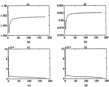
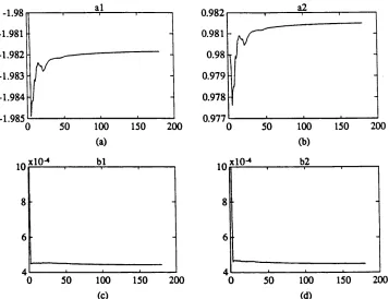
Fig. 4.8 Forgetting simulation results, X = 0.98 ... 109
Fig. 4.9 Remembering simulation results, X = 1.02... 109
Fig. 4.10 First joint simulation r e s u lts ... 110
Fig. 4.11 First joint param eters id en tifie d ... I l l Fig. 4.12 Second joint simulation results ... I l l Fig. 4.13 Second joint parameters id e n tifie d ... 112
Fig. 4.14 Backward simulation sc h e m e ... 114
Fig. 4.15 Compensated backward simulation sch em e... 115
Fig. 4.16 Step input backward sim ulation r e s u lts ... 116
Fig. 4.17 Sin(4t) input backward simulation r e s u lts ... 116
Fig. 4.18 l-cos(4t) backward sim ulation re s u lts ... 117
Fig. 4.19 2 DOF backward sim ulation r e s u lts ... 117
Fig. A4.1 Two DOF p e n d u lu m ... 120
Chapter 5 Fig. 5.1 Force control scheme ... 128
Fig. 5.2 Dynamic model of c o n ta c t... 132
Fig. 5.3 Norm al c o n ta c t... 134
Fig. 5.4 Oblique c o n ta ct... 134
Fig. 5.5 Surface c o n ta c t... 135
Fig. 5.6 Adaptive outer-loop force c o n tro l... 145
Fig. 5.7 Model for force control s im u la tio n ... 148
Fig. 5.8 Stiff environment, K = 106 ... 149
Fig. 5.9 Less stiff environment, AT = 105 ... 150
Fig. 5.10 Flexible environment, K = 104 ... 151
Chapter 6 Fig. 6.1 Task formalism of peg-to-hole ... 158
Fig. 6.2 Position displacement of a joint trajectory ... 160
Fig. 6.3 The vicinity of PUMA560 gross m o tio n ... 161
Fig. 6.4 Profiles for joint-space trajectory ... 164
Fig. 6.5 Photo to show simulation ... 166
Fig. 6.6 Initial p o sitio n ... 167
Fig. 6.7 Vicinity of destination ... 167
Fig. 6.9 Picture to show the compliant device ... 171
Fig. 6.10 Linear position se n so r... 172
Fig. 6.11 Data fittin g ... 174
Fig. 6.12 Position sensors arran g em en t... 176
Fig. 6.13 Full contact rotation co m p lian ces... 177
Fig. 6.14 Partial contact rotation com pliances... 177
Fig. 6.15 Force control configuration... 179
Fig. 6.16 Drawing of the peg and h o l e ... 182
Fig. 6.17 Peg-into-hole VAL-2 program flow c h a r t... 183
Fig. 6.18 Control strategy for assembly ... 184
Fig. 6.19 Experiment of peg-into-hole... 185
Chapter 7 Fig. 7.1 H ardw are arrangem ent of sub-sea inspection sy s te m s... 195
Fig. 7.2 Typical sub-sea structure — Y-joint ... 198
Fig. 7.3 Inspection task fo rm alism ... 199
Fig. 7.4 Structure of the supervisory control p ro g ra m s... 201
Fig. 7.5 Supervisory control program la y o u t... 202
Fig. 7.6 Man-machine in terface... 203
Fig. 7.7 Control transfer between p ro ce d u res... 205
Fig. 7.8 DDCMP program fra m e ... 207
Fig. 7.9 PumalTF structure f r a m e ... 208
Fig. 7.10 The five step fo rm a t... 209
Fig. 7.11 VAL-2 program stru c tu re ... 212
Fig. 7.12 VAL-MOD2 structure fra m e ... 213
Fig. 7.13 VAL-2 program for real-time path m o d ificatio n ... 216
Fig. 7.14 Tracking d ire c tio n ... 218
Fig. 7.15 Picture to show ex p erim en t... 219
Fig. 7.16 Fixed gains force control re s u lts ... 222
Fig. 7.17 Adaptive force control r e s u lts ... 223
Fig. 7.18 Parameters id en tified ... 224
Term D efinition
a a direction in tool co-ordinates
“i acceleration of the i+Ith joint
robot wrist acceleration
bi direction of the i-2th joint
cu element of compliance matrix
d> direction of ith link
e error between desired and real system response
f friction
U force applied to the arm from hand
force applied to ith link from i-2th link
g gravitation constant
8 vector gravitation form
Gi gravitational term in ith link
h param eter in dynamic equation of two DOF m anipulator
element of inertia matrix of the dynamic equation
i num ber of joint
Ui ith link inertia matrix
J Jacobean matrix
Ji Jacobean matrix in vector form
k stiffness of the compliant device, time series
K kinematic energy, stiffness of environm ent
Ki ith link kinematic energy
A ith link length
m mass
M mass of the environm ent
n total num ber of joints, n direction in tool co-ordinates
torque to ;th link from ith link
n a torque applied to the arm from hand
o o direction in tool co-ordinates
P*
robot w rist positionPi
i+l th joint positionQi joint angle
4t
joint angular speedr reference input
h .i + i vector representation of link i
r«-1.3 vector comprised of /-2 th joint and w rist
h a vector form present joint i to ith link centre
u direction in the link co-ordinates
T sam pling period
*i torque of ith joint
e. ith joint angular displacement
u control input
U potential energy
V viscous coefficient
Vf velocity of the ith joint
V 3 velocity of robot w rist
V , velocity of ith link mass centre
V velocity
5 , angular velocity of the ith link
-T*
CO,. angular acceleration of the ith link
y system output
1.1 INTRODUCTION
As can see from the title of this thesis, the work is concerned with two aspects of robotics research. The first is dynamic control, other than simple constant PID control, for robotic m anipulators. The other one is robotic force control m aking contact w ith the environment. The research is framed within dynamics and control i.e. mainly in mechanical aspect of robotics research.
Dynamic control is directly aimed at fast and precise performance. The simple constant gain PID controller provides sufficient performance in many elementary industrial tasks. However, the performance of such controllers decreases rapidly when dynamic effects become significant, for example, the arm m ay become unstable when moving at high speed or under high load.
capabilities in perform ing tasks where contact has to be made. Almost all the industrial robot m anipulators now commercially available are non-contact type, which greatly restricts their use. Pick and place, spot w elding and similar tasks, can be accomplished using only purely position control.
The advent of powerful, cheap and compact com puters has had as great an im pact on control systems as on other fields of engineering. M odem controller systems, w hether used in industrial process control, ship guidance or aircraft 'fly by wire' systems now almost exclusively incorporate microprocessors as the m ain computational element.
Com pared w ith its analog counterpart, digital controllers offer tw o major advantages: One is that they decrease size and num ber of components. The other is its flexibility. Digital controllers w in hands dow n over analogue controllers in this respect, as their control law and general operation m ay be altered by replacing the control programme, usually just a case of changing a instruction in a program. To alter the control law or operation of a dedicated analogue controller may require a complete redesign of the circuit, obviously som ething that cannot be carried out quickly and cheaply. Digital controllers w ith communication links m ay even be program m ed remotely over the communication link, a process known as 'dow n line loading7. One new micro-controller is designed to plug directly into the phone system to be remotely program m ed.
Digital control, especially self-tuning PID, is extensively analysed and sim ulated and used as a main control scheme in this thesis.
1.2 LITERATURE REVIEW
As a highly nonlinear, highly coupled multi-variable system, the robotic m anipulator provides one of the most challenging and active fields of research within the control community. Many modern control approaches are applied to the control of the robotic manipulator. However, these m odern control
schemes have either little practical use (e.g. lack of persistent excitation problem in the robotic adaptive control) or are too expensive as they have very complicated forms. The following sub-sections will have a review of the current research in tw o m ain topics of robotics.
1.2.1 Adaptive Control of Robotic Manipulators
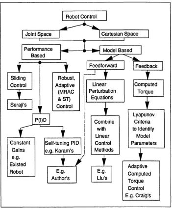
Basically there are two kinds of control scheme, one is the so called performance-based control scheme. The other is called model-based control, where the dynamic model of the physical system to be controlled are explicitly appearing in the controller. Fig. 1.1 show s the classification of commonly used robotic control schemes. Although, there exist two control co-ordinates, joint space and Cartesian space, m ost of the existing control schemes are based on the joint space. Cartesian trajectory control (and force/com pliant motion control) are achieved by closing the loop around the inner joint servo loops.
As can be seen in Fig. 1.1, the dynamic model can be used in two ways. It can be placed in the feed-forward loop to form the so called feed-forward compensation (or part of the dynamic model, usually gravitation, to form the so called partially compensation). And the model can also be placed in the feedback loop forming so called feedback linearization, i.e. so called computed torque control Craig [1989] further develop the com puted torque control m ethod by using the Lyapunov criteria to identify the m odel param eters to cover the problem of model uncertainty. The resulting adaptive computed torque control was achieved because of his research. Craig's m ethod is the m ost robust one b u t is also the m ost expensive controller because identification has to be processed together w ith calculation of robotic dynamics, which is complicated itself.
equations together w ith the m inim um variance self-tuning adaptive control strategies by Clark and Gawthrop [1975] to form his unique control scheme. But his scheme is complicated and has a central coupled form.
Robot Control
C artesian S p ace Joint S pace
Model B ased Perform ance
B ased
Sliding Robust,
Control Adaptive
* (MRAC
& ST) Seraji’s
Ir
Control P(I)D C onstant Gains e.g. Existed Roboti
Self-tuning PID e.g. Karam ’s
Feedforward Linear Perturbation Equations Combine with Linear Control Methods
i
E.g. E.g. Author’s Liu's Feedback Com puted TorqueI
Lyapunov Criteria to IdentifyModel P aram eters
I
Adaptive Com puted Torque Control E.g. Craig’sFig. 1.1 Control of robotic manipulators
The author used W ellstead's pole assignment self-tuning adaptive control for designing the control scheme. The model feed-forward compensation is used to decrease the non-linearity and coupled effect. After feed-forward
compensation, the author assumes that the system can be treated as a set of de-coupled sub-systems. So each joint can be treated individually, just as in conventional industrial robotic m anipulator control.
Performance-based m ethods are based on the assum ption that an accurate dynamic model is not always available or is difficult to calculate, especially w hen various unknow n payloads are to be m anipulated by the arm. In the unknow n payload situation, m odel-based m ethods have alm ost no effect. It is mainly for this reason that various performance-based control scheme have been developed during the last decade. Sliding-mode control, robust control and adaptive control are all good examples of these control schemes. Slotine and Li [1991], Asada [1986] and Seraji [1989] are all pioneers in the sliding mode control developm ent for robotic m anipulators. Various robust control controls UkeH~ are also applied to the m anipulator control.
The use of adaptive control for robot m anipulators is not new. It is evident that adaptive control will definitely improve the performance of robot m anipulators in terms of positional accuracy and response speed. However, industry still uses conventional simple PID controller for each joint. The main reason for this is because of the complexity of adaptive control, which affects reliability, and its high cost to implement.
Dubowsky and DesForges [1979] were the first to use Model Reference Adaptive Control (MRAC), where a continuous time single-input single-output (SISO) adaptive controller was designed for each joint of the m anipulator. This m ethod is easy to implement and has a small num ber of
computations. However it ignored the coupling betw een joints and thus
Koivo and Guo [1983], first used m inim um variance Self-tuning control developed by Clark and Gawthrop [1975] for the joint control of a robotic m anipulator (Stanford Arm). However, Koivo and Guo's m ethod is limited to systems that are open loop stable and the weighting factors P and Q in the cost function were restricted to be constants, and no rule was given for choosing them. Afterwards, there have being m any papers which improve Model Reference A daptive Control (MRAC) and Self-tuning Adaptive Control (STAC) for robotic manipulators.
Craig [1988], in his book, has a very good review of these papers, which, to sum m arise, have the following drawbacks:
1). It is still restricted to low speed configuration changing, ie slow speed manipulation.
2). Global stability is not guaranteed.
3). For slow time-varying param eters, Lyapunov stability theory can be used for MRAC and linear theory can be used for self-tuning adaptive control. 4). N one of them deals w ith the problem of lack of persistent excitation. Craig [1988] did not mention that some adaptive controllers have a centralized structure and some require extensive computation.
Refer to Fig. 1.1, it is worthwhile to single out the following people's work: Seraji [1989], Liu [1987], Craig [1988] and Karam [1989], because they stand for four different m ethods in the robot m anipulator control.
Seraji's sliding m ode control is the easiest so far as the author knows, where the controller is totally performance based and with no consideration of the m anipulator dynamics. However, in Seraji's scheme, there remains the problem of how to choose the weighted error criterion. A nd w hat is more, in sim ulation the control inputs have show n high chattering phenomena.
Liu [1987] used N-E dynamics equation to make feed-forward compensation, then linearize the dynamic equation to derive a linearized perturbation equation. The param eters of the perturbation equation are identified, which
are then used for updating the controller's gains. His m ethod implies that a rather accurate dynamic model is available and has the centralized form which is very complicated. Liu's m ethod can be viewed as a combination of the m odel based and adaptive control.
Craig [1988] combine the com puted torque and adaptive control for robotic m anipulators. The L-E dynamics equations are used for calculating the feedback compensation w ith a position and velocity feedback loop. W hat's more, the param eters of the L-E equations are identified using the Lyapunov criterion to cover the problem of m odel uncertainty. His m ethod is the m ost robust one w ith only the dynamic equation structure being needed, b u t it is also the m ost complicated.
The self-tuning m ethod that has show n the m ost prom ise for m anipulator control is an adaptation of W ellstead's [1979] pole-placement self-tuner by Leininger [1983]. Karam [1989] recently show ed a very interesting adaptive controller which has the same form as Leininger's for robotic m anipulators. Karam 's controller is a simple PID structure and the second order dynamic m odel is assigned to each joint of the robotic m anipulator. Because of such a simple choice the explicit relationship betw een the process param eters and the PID controller's gains can be acquired. His scheme is only an im provem ent of the traditional PID controller which is widely accepted in industry. The difference is that the dynamics of the robot m anipulator are taken into account by resolving the process param eter into the designing of the PID controller using an adaptive strategy. In an early work (Wang [1991a]), this kind of controller has been simulated.
1.2.2 A daptive Robotic C om pliant M otion C ontrol
M anipulation fundam entally requires the m anipulator to be mechanically coupled to the object being m anipulated, the m anipulator m ay not be treated as an isolated system.
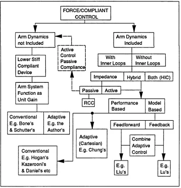
As show n in Fig. 1.2, two m ain groups can be distinguished: one group (first group) takes the compliant motion as a system, and the dynamics of contact include both m anipulator itself and environm ent. The other group (second group) applies a low stiffness compliant end-effector m ounted at the robotic m anipulator's end-effector, so as to ignore the m anipulator's dynamics.
FORCE/COMPLIANT CONTROL 1 Lower Stiff Compliant Device
I
Arm Dynamics i Arm Dynamics
not Included
r J - , Included
Arm System Function a s Unit Gain
Active j
Control I
P assive j Compliance]
I
With Inner Loops
Im pedance
■— | P assive
Without Inner Loops
Hybrid
Active
Both (HIC)
RCC
Conventional Adaptive
E.g. Bone’s E.g. the
& Schutter*s Author’s
i
Adaptive (Cartesian) E.g. C hung's
Perform ance B ased Model B ased Feedforward Feedback Combine Adaptive
1 r Control V
Kazerooni’s E.g. E.g.
& Daniel’s etc Liu’s Lu’s
Fig. 1.2 Force control category
In C hapter 5, more detail will be given to the second group. The first group can be further divided according to w hether there is an inner high-bandw idth loop (Daniel [1989]), or not, as An [1989], Liu [1988], Epping [1986], Seering [1987] and Youcef-Toumi [1987]. W ith an inner loop, it is assum ed that the force control loop is closed around some higher-bandw idth inner loop, such as a position controller (Kazerooni [1989], Stepien [1987], W hitney [1976], and Paul [1987]). A review of the different control architectures in which force feedback appears is presented by W hitney [1987].
Master and slave m anipulators can be dated u p to 1940s. Later in 1950s, force-feedback was applied (Whitney [1985]). Time delay of as little as 250 milliseconds will cause these systems to be unstable. At the turning of 1970s, research turned to replacing the hum an operator w ith a computer. All the approaches depended on people to form ulate the details, and those systems that were tested experimentally encountered the stability problem. The problem has been m itigated by the use of m ore sophisticated control algorithms, faster computation, and flexible sensors, b u t as yet no automatic generation of strategies has been achieved.
Force feedback, from its very beginning, is in the operational space, which is especially true w hen a w rist force sensor is going to be assembled at the m anipulator end-effector. W ith this feature, force control is totally different from joint servo control. When the m anipulator dynamics are taken into account, force control is coupled with the joint of the m anipulator being used w ith each joint contributing to the overall contact forces/torques. So co-ordinate transformations between operational space and joint space are required within each sam pling period.
revolute joints, with no speed reduction gear, i.e, the link is driven directly from the actuators. His Cartesian force control scheme is based on the dynamic system of the robotic m anipulator m aking contact w ith the environm ent. The whole control scheme is open-loop w ith no force feedback. The contact force is m aintained on the assum ption that the joint torque can be controlled precisely, which is m ade possible on the Direct Drive Arm developed at MIT.
An [1989] succeeded in controlling the contact of his 2 DOF robotic m anipulator w ith the environment. A ttention has to be draw n to some parts: 1). The simplicity of the m anipulator configuration he chose results in a simple transform ation between co-ordinates. 2). There is no wrist-force feedback, so the stability problem becomes less im portant.
It is for these reasons that m any force control schemes in the literature still use the inner higher bandw idth loop. The task space operational path and force control is accomplished by an outer-loop force/position control loop which are closed around the inner-loop. However, in these schemes, under existing com puter power, force feedback can not be calculated quickly enough. Taking the PUMA560 industrial robotic m anipulator as an example, force feedback can only be com puted at the sam pling rate of 36 H z, ie a sam pling period of 28 ms. This time period is too long for the real-time force control implementation. The m anipulator bounces against the environm ent uncontrollably. A compliant end-effector was assembled betw een the robot end-effector and its environm ent to solve the stability problem.
The effect of using a lower stiffness com pliant device is to greatly reduce the whole system stiffness, thus reducing operational speed and cause other side-effects on system performances as will be discussed in Chapter 6 . It is highly desirable that the system can be operated in a stable w ay w ithout a compliant device. Purely Cartesian force control scheme in the operational space w ithout an inner-loop needs a very powerful com puter, so as to increase sam pling rate.
Daniel's [1989] work suggested that inner-loop force feedback should be added other than position feedback alone. His group has done a lot of work in force control w ith force (torque) feedback w ithin each joint servo. In their research, they found that velocity feedback m easured by a tachogenerator, rather than calculated from the position differences (encoder based, common practice of industrial robots), is crucial for the whole system stability in the extremely low speed m anipulation w hen a robotic m anipulator has m ade contact w ith its environment.
However, for the PUMA560 robotic m anipulator, there is an anti-backlash m echanism which introduces compliances betw een joint m ounted strain gauge (for m easuring force/torque) and the motor. This results in a slip /stick phenom ena w ithin the drive, not observable from the m otion of the robot, which generates high frequency signals from the strain gauges. As soon as the m otor moves, stick/slip injects high frequencies into the anti-backlash mechanism which then resonates. The internal resonance is uncontrollable due to the slip /stick non-linearity betw een the m otor and the mechanism and can send a strain gauge based inner-loop controller unstable. This phenom ena restricts the bandw idth of the inner-loop controller to below the resonant frequency and thus limits the am ount of sustainable outer loop feedback.
O ther schemes to improve the inner-loop exist, and are not discussed here in great detail. It is rem arked here that no differences are given to Cartesian and operational space (task frame) compliant (force) control schemes, as the m ain purpose is to define the differences of these control schemes from the common joint servo control systems. The essence of Cartesian and operational space hybrid control schemes is that the co-ordinate transform ations are now within the control servo-loop.
named: Stiffness control; D am ping control; Hybrid force-position control; Im pedance control, etc. This is still confusing as there are m any control schemes for the m anipulator itself, like P(I)D, adaptive and sliding m ode etc. (refer to the form er section). For this reason, it is suggested that w hen a force control m ethod is referred to, it should also refer to the arm position control m ethod as well, and so suggested nam es can be Stiffness-P(I)D, D am ping-Adaptive and Hybrid-P(I)D force control etc.
According to the w ay force-feedback is incorporated into the m anipulator's position servo, two main force control approaches can be distinguished: (1) H ybrid, and (2) Impedance control. In the later m ethod, the force signal is transferred as position or velocity commands, which are then in p u t to the m anipulator position servo and the m anipulator rem ains as a position controlled device.
Im pedance Force Control
Im pedance force control is a general approach to robot m otion and force control that attem pts to make a m anipulator behave as a m ass-spring-dashpot system (Hogan [1985]), whose param eters (inertia-stiffness-damping) can be specified arbitrarily. A simple example w ould be to give a robot arm spring-like characteristics. A large spring constant results in a stiff arm. Position and force control are considered tw o forms of im pedance control. Position control implies very high impedances, while force control implies the opposite.
Im pedance control has not been im plem ented in its full form, b u t rather in some simple forms like stiffness or dam ping control. Im pedance control does not specify desired forces or positions, b u t rather desired dynamic relationship betw een force and position, in other w ords mechanical stiffness or "impedances", w ith fairly slow motions.
Remote Central Compliance (RCC) is a typical passive compliance, capable of quick response, b u t its applications are necessarily limited to very specified tasks - RCC, for instance, can only achieve peg-into-hole problem.
A program able active control, by contrast, w ould allow the m anipulation of various types of compliant motions by controlling the whole arm impedances. In the other w ords, w e can get the desired end-point stiffness by appropriate controller design of each joint-servo to acquire the desired joint stiffness. In this sense, the m anipulator can be seen by the environm ent as a spring and damping.
ARM
Sensor
Fig. 1 3 Impedance force control scheme
As show n in Fig. 1.3, force is transferred to position and velocity w ithout desired force appearing in the structure. Force control is accomplished by controlling the position. If Kv is chosen to be zero, then it has the structure of stiffness control, likewise, if Kp equals to zero, the controller is simplified to dam ping controller.
lim ited by the stiffness of the environm ent. For example, w hen a m anipulator is contouring a stiff object, the environm ental stiffness varies between extremely stiff and extremely soft according to w hether contact is m ade or not. In order to reduce the stiffness and to avoid oscillation of motion, heavy dam ping m ust be applied, and this dam ping determ ines the speed at which the m anipulator follows the object w hen the contact is broken. It has also been realized that stability can be m aintained if some compliance, which m ay be derived from a force sensor or an end-effector, is inserted between the m anipulator and an object, since this reduces the environm ental stiffness for the joint servo. However, it also reduces the advantage of the stiff servo rigidity of the m anipulator and m akes it impossible to achieve a combination of rigid m otion and soft motion along different axes.
Im pedance control has been im plem ented in m any forms. In its sim plest form it can be considered as a generalization of dam ping and stiffness control schemes. In this form, it is essentially a PD position controller, w ith position and velocity feedback gains adjusted to obtain different impedances.
Hybrid Force Control
Raibert and Craig [1981] first suggested this m ethod for force control, in which force and position are both added to the joint servo of robotic m anipulators individually. Forces are not transferred as position com m ands, b u t applied directly to the joint servo. That is to say, even if there is no motion, the joint servo m ay be asked to provide a torque to m aintain a pre-specified end-effector contact force.
In Raibert and Craig's [1981] original hybrid force control controller, only proportional gain is present. To im prove control property, velocity and integration feedback are added as in Fig. 1.4. Inverse Jacobean matrix is presented in the control structure, which, according to A n [1989], is the m ain reason for the hybrid controller's instability.
The theory backed hybrid force control is that the force-controlled directions and the position controlled direction in the operational space are com plem entary and orthogonal w ith each other. So the force-controlled directions can be grouped as a sub-space, as can the position-controlled directions. Both of these sub-spaces contribute to the joint servo, and their dem ands are transferred to joint space by calculating the inverse Jacobean transform ation matrix. The position servo is supposed to be infinitely stiff and rejects all force disturbances acting on the system. Likewise, an ideal force servo exhibits zero stiffness and m aintains the desired force application regardless of position disturbances.
s — ► J1 -► P(I)D
l-S ---- ► P(I)D
ARM
Fig. 1.4 Hybrid controller
As described in the former section, it m ay be useful to be able to control the end-effector to exhibit stiffness other than zero or infinite. In general, we m ay w ish to control the mechanical im pedance of the end-effector. In hybrid control schemes, it is assum ed that the environm ent the robotic m anipulator is to make contact w ith is very stiff. In m any applications this assum ption is not true, so hybrid impedance control is used.
Hybrid Im pedance Control Scheme
im portance of m anipulator impedance. Im pedance control considers the effects of m anipulator impedance on ro b o t/en v iro n m en t interactions. W hen perform ed in task space, a know n im pedance can be m aintained for all configurations. It is considered, how ever, to be solely a position-controlled scheme, w ith small adjustm ents m ade to react to contact forces. Positions are com m anded, and impedances are adjusted to obtain the proper force response. N o attem pt is m ade to follow a com m anded force trajectory and any distinction betw een force-controlled sub-spaces and position-controlled sub-spaces is ignored.
How ever, in hybrid force control, system stability is a problem. It is also w orthw hile to point out that hybrid force control is only suitable for a stiff environm ent (as will be seen in the sim ulation present in C hapter 5). If the environm ent is flexible w ith noticeable displacem ent w hen force is applied, then force-controlled and position-controlled direction are difficult to distinguish and are not orthogonal to each other.
Several researchers have tried to combine both im pedance and hybrid control schemes to form the so called H ybrid Im pedance Control (HIC). The basic idea of HIC is that in the force controlled directions, position feedback is introduced, and in the position controlled directions force feedback is introduced. Fig. 1.5 shows one of the HIC control schemes:
Robot
Kp1+Kd1+Ki1
Fig. 1.5 Hybrid impedance control scheme
This is the general form of the H ybrid Im pedance Control (HIC) scheme. If position gains in the force-controlled direction are zero, and force feedback gains in the position-controlled directions are zero, then the H ybrid control scheme is obtained (different from the original one). If force control servo does not exist, then a kind of impedance control results. As show n in Fig. 1.5, inverse Jacobean matrix does not appear in the control loops (transpose Jacobean m atrix does).
Adaptive Cartesian Com pliant Control
As stated before, joint space force/torque -feedback is undesirable because of the noise and slip/stick phenom ena (for PUMA560, probably not in DDArm). H ybrid force/position control shows coupling betw een these two loops, which affects the arm performance. Most of the hybrid or hybrid im pedance control scheme supposes the control is to be accomplished in the robot operational space, and there is no inner higher bandw idth position/velocity feedback loop.
--- 1
■^Identification
P(I)D 1 T KIN(q) ARM q ^ . Control
Pseudo
Input Input
or
Servo vi(q)
Task space Joint space
X or F
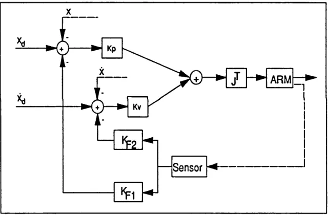
Fig. 1.6 Adaptive force control scheme
and Leininger [1990] used W ellstead's pole placem ent self-tuning adaptive control strategies for task level force control. His controller is of hybrid structure and there is no feed-forward com pensation in the control scheme. Both schemes identify the dynam ic relationship betw een the Pseudo-input and the o u tp u t task-level forces/positions, w hich are m easured at the wrist.
C hung and Leininger [1990] had also im plem ented their control scheme on a PUMA600 robotic m anipulator. The task specified is to m ove a load of 2.27
kg around a vertical square w ith round comers. The actual w rist
position/orientation of the end-effector w ith respect to task co-ordinate, w hich is fixed in Cartesian co-ordinates in this case, was calculated in real-time from the joint encoder. The sam pling time required was determ ined to be 28 ms. Experimental results show further necessary refinem ent for real-time industrial applications, m ainly due to the large sam pling period (compared w ith 0.875 ms in the joint servo feedback). Lu [1991] injected Craig's [1986] m odel based adaptive control scheme to H ogan [1985]'s im pedance control to form his force control scheme.
1.3 OBJECTIVE OF THIS RESEARCH
The objective of the research is to obtain a better understanding of the dynamic and force control properties of a robot m anipulator. One end goal is to autom ate a sub-sea inspection task, which is one of the overall aims of the Automatic Control Group, U niversity College London. The present task to move an inspection probe along the inspecting surface is done by human-beings. Robotic com pliant m otion control is necessary for a m anipulator to carry out this task automatically.
W ith over ten year's experience in autom atic inspection, the Autom atic Control G roup has gained a w ide range of expertise in this field, especially in sub-sea or such ill-organised environm ents. C hapter 7 will have a detailed description on this subject. Usually there are four stages in sub-sea inspection operations.
The actual inspection operation needs the probe to m ake contact w ith the w orking object This is a very good application for robotic compliant motion control to autom atic this process. The w ork present in this thesis contributes to the last stage of sub-sea inspection.
A nother objective of this research is to investigate ways of m aking the traditional industrial robot m anipulators do as m any tasks as possible.
1.4 SUMMARY OF M A IN CONTRIBUTIONS
As the result of this study, a few contributions are sum m arised as follows: 1). A new sim ulation scheme for the control of robotic m anipulators was
developed for the first time. This scheme can m ake direct use of N ewton-Euler dynamic equations, which have traditionally been thought of as inconvenient for sim ulation of robotic m anipulators.
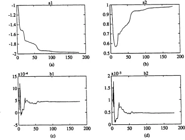
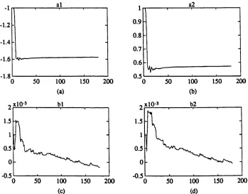
2). An approxim ate recursive least square identification was assessed and judged. Its use for robotic m anipulator w as sim ulated extensively. This simplified m ethod can greatly reduce the m athem atic calculations. Simulation show s that the control effect can be m uch im proved as the chattering control input phenom ena will disappear by letting the forgetting
be
factorslightly great than one.
3). A new self-tuning adaptive PID controller, w ith new explicit relationship w ith process param eters, was w orked out. Tustin's bi-linear transform was used to acquire the digital PID controller from its analogue counterpart, w ith adding an extra param eter. A general discrete transfer function for the second order system was used to represent the process.
5). Robotic assembly was attem pted using the PUMA560 industrial robotic m anipulator. It has been succeeded in p u ttin g a peg into a hole with m axim um clearance 0 . 0 2 m m at a reduced speed.
1.5 ORG ANISATION OF THE THESIS
The whole PhD thesis consists of eight chapters. C hapter 1, as usual, is devoted to introduction, w hich has a full review of w h at people have done in this field of research, discussion on objective of this research and m ain contribution as a result of this research.
Chapter 2 contributes to the kinematics and dynam ics of a robotic m anipulator — PUMA560. A new solution in the Autom atic Control G roup, UCL, to the kinematic of PUMA m anipulator is described. This solution makes uses of both analysis and geom etry together, instead of heavy m atrix m anipulation, to solve the kinematics problem. A new dynam ics m odel for PUMA560 was w orked out and described in C hapter 2.
C hapter 3 deals w ith self-tuning adaptive control theory. A n approxim ate RLS identification m ethod was introduced and assessed. A new self-tuning PID
a
digital controller based on general discrete transfer function was developed.
A
C hapter 4 is mainly about the practical application of w hat described in Chapter 3 for robotic m anipulators. It is found that by sightly increasing the forgetting factor to be larger than 1 it is possible to get rid of the control in p u t chattering effect.
C hapter 5 is about the compliant m otion control theory. Coupled concept for surface contact was introduced for the first time. M ethods to im prove contact quality and tracking ability has been investigated.
C hapter 6 is devoted to the application of adaptive com pliant motion control for robotic assembly, ie peg-into-hole problem. A com pliant device and its feature are described and analysed. ^Control strategy for assembly has been discussed and the practical experim ent was described.
C hapter 7 is for the application of adaptive com pliant m otion control for robotic sub-sea inspection. It is concluded that adaptive com pliant m otion can largely im prove contact quality and tracking ability.
2.1 IN TRO D U CTIO N
Dynamics of a robotic m anipulator are introduced in the next few paragraphs to give a d e a r review of w hat people have done in this field of research and w h at has been done in this project.
From the point of view of dynam ics, the robotic m anipulator is a highly nonlinear, highly coupled and param eter changing m ulti-variable system. Because of this, the control of robot m anipulators is difficult. N ow adays dynam ic control m ethods either ignore or make only limited com pensation for the variation of inertia and payload, or coupling betw een joints, which thus lead to the degradation of response velodty and accuracy. However, nonlinear control m ethods, such as, torque calculating and nonlinear feed-forward, usually need a more accurate dynam ic m odel and at the same time, a m ore complicated control structure, thus incurring higher costs in com putational b urden w hen p u t to practical use.
Basically there are tw o ways to form ulate the dynam ic equations of a robotic m anipulator, one being the New ton-Euler (N-E) m ethod; the other is the Lagrange- Euler (L-E) m ethod. Because of L uh's w ork [1980], the com putation complexity of the N-E m ethod has been reduced dram atically, from 0 ( n 4) to
O(n) (n is the num ber of joints). A comparison has been m ade in Table 2.1 (cf. Fu [1987] ppl32). This is accomplished by setting u p the calculation in recursive from and by expressing the velocities and accelerations of the links in the local link frames of reference. Nevertheless, N-E equations have their ow n inherent draw backs in that they are difficult to use in the designing of the control system and in simulation.
The L-E equations, on the other hand, provide explicit state equations for robot m anipulator dynamics and can be utilized to analyse and design advanced joint-variable space control strategies. The only defect of L-E equations is
their com putational inefficiency which arises partly from the 4x4
hom ogeneous matrices and the inverse Jacobean matrix. Hollerbach [1980] exploited the recursive nature of the L-E form ulation. However, these recursive equations destroy the "structure" of the dynam ic m odel which is quite useful in providing insight for designing the controller in state space (Fu [1987] pp84). For state space control analysis, one w ould like to obtain an explicit set of closed form differential equations (state equations) that describe the dynam ic behaviour of a m anipulator. In addition, the inertia and coupling forces in the equations should be easily identified so that an appropriate controller can be designed to compensate for their effects.
Table 2.1 Comparison of dynamics computational complexity
A pproach L-E M ethod N-E M ethod
Multiplications 128/3 n4 + 512/3 n3 + 739/3 n2 + 160/3 n
132 n
Additions 98/3 n4 + 781/6 n3
+ 559/3 n2 + 245/6 n
l l l n - 4
robot m anipulators. The last three joints of m ost industrial robot m anipulators are coincident at a point, the robot m anipulator's kinem atics can be analysed separately (Fu [1987]). H orak noticed that the sam e thing existed in the dynam ics analysis of the robotic m anipulators, by separating the robot m anipulator into tw o parts. The first p art com putes the inverse dynamics of the first three links using the L-E equations expressed in symbolic form and the second p art com putes the inverse dynam ics of the h an d (i.e. the last three links) using the N-E equations, also in symbolic form.
The symbolic m ethods fully exploit the particular kinem atic and dynam ic structure of a given m anipulator and elim inate unnecessary arithm etic operations, either inherent in the form ulation of kinem atic and dynam ic equations (e.g., the sparsity of m atrices and vectors) or arising from the
geometrical and inertial param eters of the m anipulator (e.g.,
parallel/p erp en d icu lar joint axes, zero-length links or sparse inertia tensor) (Kircanski [1988]). Also the com putations related to the first p art of the m anipulator are based on classical (non-matrix) L-E equations. There are no rotation matrices, which leads to reduction in the com putation burden of the dynam ic equations, as will be show n in next sections.
To sum m arize, the author here included the following strategies to reduce the com putation complexity:
1). To divide the robot m anipulator into tw o part, an arm and a hand. 2). To use vector m anipulation instead of matrices.
3). To use the symbolic form, and m aking full use of the PUMA configuration.
2.2 KINEM ATICS OF THE PUMA560
The position (forward and inverse) of the PUMA can be decided by combining geom etry and analysis together (Fu [1987]). An effective program has been w ritten for the PUMA560 robot m anipulator kinematics in the Autom atic Control G roup, w ith all the calculations being based on vector m anipulations and no matrixes being involved. The key points are:
1). To separate the robot m anipulator into tw o parts, an arm and a hand, calculating the kinematics of each individually.
2). To calculate, on-line, the direction of each joint axes bH (in this chapter, joints are num bered as 0 ,1 ,..., 5 while links are num bered as 1 ,2 ,..., 6) and the direction dt of each link recursively, using the technique of one vector rotating about the other.
2.2.1 Vector Rotation
M athem atics tools used for kinem atics analysis is m ainly vector rotation, and is outlined here for necessary background.
b: a vector (e.g. joint axis)
d: a vector rotating around b
d': new place o f d
Fig. 2.1 Vector rotation
PROCEDURE rotVec(VAR pvec, nvec: VECTOR; VAR alpha: REAL): VECTOR;
nCP:= crossP(nvec, pvec); (’‘C ross product of tw o vectors*)
pDotN:= dotP(pvec, nvec)*(1.0 - cos(alpha)); (*Dot product of tw o vectors*)
FOR i:= 1 TO 3 DO
pvec[i]:= pDotN*nvec[i] + cos(alpha)*pvec[i] + sin(alpha)*nCP[i] END;
RETURN pvec;
w here crossP and dotP are tw o separate routines for doing vector cross m ultiplication and dot m ultiplication respectively.
2 .2 . 2 P osition-O rientation K inem atics of a Robotic M an ip u lato r
The first three degre^of freedom decide the position of the PUMA560 robotic m anipulator (can be extended as a general rule to other robotic m anipulators). The last three degree of freedom s decide the orientation of the PUMA560 robotic m anipulator end effector. If the displacem ent of each joint of the robotic m anipulator is decided, the position and orientation of the arm can be uniquely decided (forward kinematics). The other w ay round is not true, that is, if the position and orientation of the arm is decided, the joint angles can not be uniquely decided (inverse problem).
Forw ard K inem atics of PUMA560
Forw ard kinematics m eans deciding the m anipulator position and orientation according to the joint angles. As stated before m ost industrial m anipulators can be divided into an arm and a hand, which can then be treated individually.
(1). Position
Supposing the angular displacem ents of joint 1,2 and 3 are know n, as show n in Fig. 2.2, then w rist position P3 can be calculated recursively.
P3 b2
d3 P 2
b l
bO P1
PO
Fig. 2.2 Calculate wrist position
In Fig. 2.2, bi_t (bold characters in text stand for vectors too in this thesis) is
i-1 th joint direction, d, ith link direction and P{ is ith joint position. P3 is called the w rist position. b0 is coincident to one (usually z) axis with the w orld coordinate and is not changing.
Rotating the first link around b0 in a angle 0j, the position P t and orientation
bt of the second joint can be decided using vector rotation described in the form er sub-section. A t the same time the orientation b2 of joint 3 can be decided as b2=bv because of the special PUMA geom etry. By rotating d2 around bv P2 can be calculated, and so is the w rist position P3. This seems straight forw ard and refer to Lovell [1990] for a detailed description.
(2). Orientation
t: tool-coordinate
Fig. 2 3 Calculate orientation
A sim ilar calculation of the orientations of the last three joints can be m ade by using vector rotation. Once w rist position P3 an d direction of link three d3
have been calculated in the form er part, the robotic end-effector, i.e. tip-position and tip-orientation (or b ^ can be decided recursively. As show n in Fig. 2.3, direction of joint 5, bA can be calculated by rotating it, in 6 4, around joint 4 direction b3, which equals to d3 (Fig. 2.2). Direction of joint six b5/ which is the sam e direction as the direction of joint six, can be calculated by rotation it around b4 in the angle 05. A nd lastly, the tip-position and orientation can be calculated.
Inverse K inem atics of PUMA560
Given a position/orientation in space, the calculation of the corresponding joint angles is called the inverse kinem atic problem . The inverse problem is n o t so straight forw ard as the forw ard kinem atics problem , w ith m u lti-so lu tio n s.^\lu lti-so lu tio n problem is solved by choosing a specific configuration convenient for arm m anipulation.
As stated before, the m anipulator can be divided into tw o parts, an arm and a hand. Because of this, this research uses geom etry together w ith sim ple
analysis m ethod to solve the inverse problem . N o 4x4 hom ogeneous m atrix transform ation is involved. The tim e for inverse problem is kept to a m inim um .
G iven a position and orientation to the end-effector of a robotic m anipulator, the w rist position P3 can be calculated, w hich is then used to derive the first three joint angles. The last three joint angles can be derived by the tip-orientation.
(1). Position
"A" Direction (X-Y Plane)
*B" Direction
P3
P3
PO
Fig. 2.4 Calculate first three joint angles
Suppose the w rist position P3 is specified. N ow , it is needed to decide the angles of joint 1,2 and 3. In Fig. 2.4, the left-hand side is the projection of Fig. 2.2 in the "A" direction and the right-hand side, projection in the "B" direction. A nd Lj is the first link length, P3 is w rist position projection seeing from "A" or "B" direction, the dashed-line show the initial state and the solid line, the new state of the m anipulator.
the position of the second joint P v The first joint angle, w hich is the angle betw een initial link 1 and new link 1, can be easily solved using geometrical analysis.
The right-hand figure in Fig. 2.4 show s the projected image of arm seeing from direction "B". This is a plane w hich is perpendicular to link 1. Because of the PUMA special configuration, link 2 an d 3 will be in this plane — called the "S" plane. W hat has to be pointed o u t is that the PUM A configuration is chosen as concave shape, as show n in initial shape in the right-hand figure. This configuration is suitable for u p p er operation. H ow ever, in this project, the robotic m anipulator is m ainly used to d o low er operations. The configuration is then chosen as a convex shape.
The angular displacem ents of joint 2 an d joint 3 are calculated as following:
P3 in the "S” plane is know n, and P2 is decided in the first step as described. Taking P v L2 and P* L3 as the origins and radii , d raw tw o circles, which will have tw o cross points. Choose one of the cross points as position of joint 3, P2, according to the configuration required as show n in the figure. The angular displacem ents of joint 2 and 3 are calculated in the sam e w ay as described in the case of joint 1.
(2). O rientation
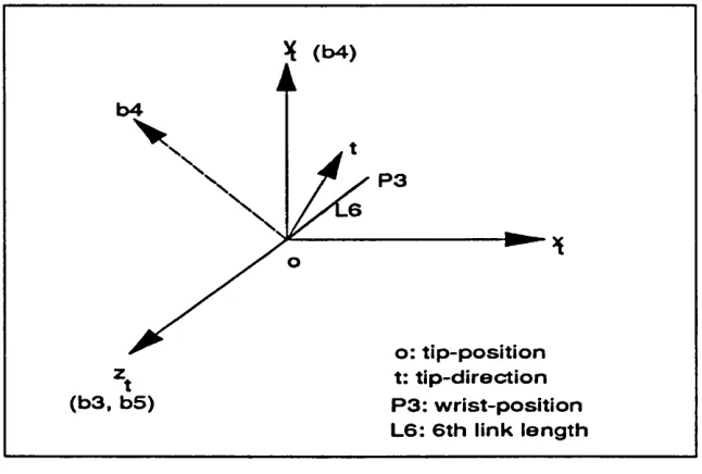
Given an orientation in space, calculating the joint angles of the last three joints of PUMA560 is called the orientation inverse problem . This problem is more difficult than the form er one. R edraw ing Fig. 2.3 by rotating the tool-coordinate 90 degrees around its y t axis, w e can get the following Fig. 2.5.
X <b4)
b4
P3
o: tip-position t: tip-direction z.
't
(b3, b5) P3; w rist-position
L6: 6th link length
Fig. US Calculate last three joint angles
w here t is the tip-direction specified, initial b5 an d zt are coincident, and so are b4 and y t. The angle betw een vector t and axis b3 decide the required an g u lar displacem ent of joint 5. The cross p ro d u ct of vector t an d axis b3 is the n ew axis of joint 5, b4. The angle betw een new and old axis of joint 5 decide the angular displacem ent of joint 4. A piece of MODULA-2 program for doing this is listed below:
Angle5:= acos2(dotP(tipDirect, b3), 1.0); (•Calculate angular displacement of joint 5*)
b4:= crossP(tipDirect, b3); (•Calculate new axis of joint 5*)
Angle4:= acos2(dotP(b4, b4Init), 1.0); (•Calculate angular displacement of joint 4*)
2.2.3 M otion K inem atics of a R obotic M an ip u lato r
W hen dealing w ith arm dynam ics, the velocities an d accelerations of each joint have to be calculated to judge the dynam ic response, from which suitable controllers can be assessed to acquire the best perform ances.
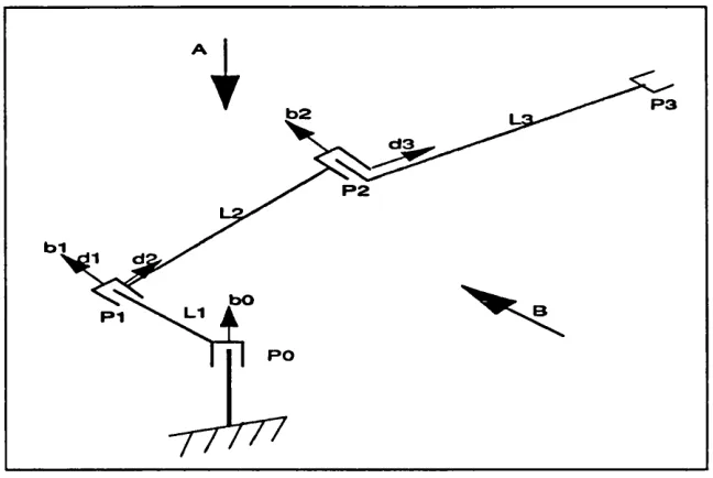
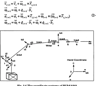
For sim plicity, a line diagram of the PUMA type robot m anipulator is draw n as Fig. 2.6. A recursive equation can be obtained as follows (Asada [1986]):
vi + 1 = v . + 3 i+1 x ri t i + 1
o ,+i = a , + 3 u , + x(G>i+, x r ,,i+l) (2_1)
3 i+, = 5 , + (?itl • 6 , + (0, x, } i + 1 •
b 4 b 2
d 3 linl bS
b3 W rist
Iink2 d 2
H an d C o o rd in a te bO
d1
b5
Fig. 2.6 The coordinate systems o f PUMA560
For the PUMA, all the joints are revolute types, so w e can easily derive from equation (2 -1) the following equations:
C0t = I <?i-*.•-!
i=i (2-2)
v»= 'L q i b i_
> = 1
The acceleration of each joint an d the angular acceleration of each link can be obtained by differentiating equations (2 -2). As can be seen in the next section, it is necessary to give the velocity an d acceleration of the w rist (i.e. tip of the third link):
V ,= £ < 3 W i i = l
O j= » * 1
(2-3)
w here / , is elem ent of Jacobean m atrix and,
S’i- , = C0i_, x ^ . . ,
k is the kth joint, and
= ^>,* = vjk- v i . 1 (2-4)
2.3 DYNAM ICS M ODEL OF THE PUMA560
N 4 v 3 ,a3
In this section the dynam ics equations of the PUMA type robot m anipulator will be derived based on H orak [1984]'s schem e of separating the m anipulator into tw o parts, using the non-m atrix form of the L-E equations in sym bolic forms.
As show n in Fig.2.7, if v3and a3(2-3) are evaluated, the dynam ics of the second p a rt can be decided by the recursive N-E equations, th u s f 4 and N 4 can be calculated ( H orak [1984]). The dynam ics of the first p a rt can be exactly com puted if the force (/*) and the m om ent (N4) applied on it b y the second p a rt are know n. The idea of H orak's can be expressed by the follow ing steps: (1). Evaluate the velocity and the acceleration of the wrist.
(2 ). C om pute the dynam ics of the second p a rt of the m anipulator, i.e., links 4,5 and 6 . This com putation can be perform ed exactly once the results of the step one are available. A t this p o in t the torques of actuators 4,5 and 6 are available, an d so are f 4 and N 4.
(3). C om pute the dynam ics of the first p a rt of the m anipulator, i.e., links 1 , 2 and 3, excluding the contribution d u e to the force an d the m om ent the second p a rt of the m anipulator applies on link 3.
(4). A dd the dynam ic effects of the second part.
2.3.1 Dynamics of the Second Part
The recursive N ew ton-Euler equation is as following:
—• (
f t -i.i 1 • g - m, • ve, = 0
N i-i.i-N, . l + 1 + x j U *7,-,., - M <W xm,) = 0 (2-5)