RESEARCH ARTICLE
VOLUME EQUALIZATION METHOD FOR LAND GRADING DESIGN: VARIABLE SLOPED GRADING
IN ONE DIRECTION AT RECTANGULAR FIELDS
*Yasar AYRANCI
Mugla Sitki Kocman University, Datca Kazim Yilmaz Vocational School, 48900 Datca-Mugla, Turkey
ARTICLE INFO
ABSTRACT
This paper presents the principles of a new method for variable sloped grading in one direction that is adapted from Ayranci and Temizel (2011) which has been developed to perform land grading design for uniform sloped grading in one direction. The main goal of this method is to minimize the volumes of earth work required for acceptable smooth surface. The method based on the assumption that the before and after grading the soil volumes measured from a reference elevation are equal. The method eliminates the need for trial and error procedures. According to the results of the application of the complete design procedure to a hypothetical area about 2.21 ha, the method is accurate in rectangular fields.
Copyright©2017,Yasar AYRANCI. This is an open access article distributed under the Creative Commons Attribution License, which permits unrestricted use,
distribution, and reproduction in any medium, provided the original work is properly cited.
INTRODUCTION
A significant amount of water (20 to 25%) is lost at the time of surface irrigation during its application to the crops because of uneven land level of the fields and inappropriate farming practices (Bansal et al., 2014). Surface irrigation methods depend on gravity and slope that make the water flow in a field (Jat et al., 2006). The preparation of the field surface for conveyance and distribution of irrigation water (Brye et al., 2005; Brye et al., 2006) is as important to efficient surface irrigation as any other single management practice the farmer employs. There are perhaps two land leveling philosophies: (1) to provide a slope which fits a water supply; and (2) to level the field to its best condition with minimal earth movement and then vary the water supply for the field condition. The second philosophy is generally the most feasible. Because land leveling is expensive and large earth movements may leave significant areas of the field without fertile topsoil, this second philosophy is also generally the most economic approach (Cazanescu et al., 2010). Land topography is of great factor for selection of surface irrigation methods. When this factor is not considered, some problems such as water loss, soil erosion and leaching of useful nutrients resulting yield reduce would occur. A successful application of surface irrigation methods and high irrigation performance depend mostly on land leveling project which is crucial for land preparation and
*Corresponding author: Yasar AYRANCI,
Mugla Sitki Kocman University, Datca Kazim Yilmaz Vocational School, 48900 Datca-Mugla, Turkey.
appropriateness for irrigation (Demirtas and Demir, 2011). Land leveling is the first step for better land development (Chilur et al., 2016). Precision land leveling can help the farmers to utilize the scarce land and water resource more effectively and efficiently towards increased crop production (Naresh et al., 2014) also, it increases yields and cultivable lands and reduces delivery losses (Sharifi et al., 2014). The purpose of the land leveling projects is to determine the most suitable leveling plane to the natural topography, taking into account the slope grades required by the irrigation method (Yildirim, 2008).
The effective application of surface irrigation methods is directly related to specific land surface properties. For example; border irrigation method requires constant slope grading in one direction, furrow irrigation method requires variable slope leveling in both directions etc. Reviewing of the literature indicates that much data exist except (Shih and Kriz, 1971) who proposed a method (Symmetrical Residuals
Method) to grade lands that allows for uniform or nonuniform
slopes in both directions on application of variable sloped leveling in one direction. According to the Scallopi and Willardson (1986), the Symmetrical Residuals Method for land leveling is still considered too laborious for general use. Nowadays, laser leveling applications are getting widespread (Rickman, 2002; Zimmermann et al., 2005; Cazanescu et al., 2010; Bansal et al., 2014; Chilur et al., 2016). This research introduces the principles and an application at a hypothetical area of the variable sloped grading method in one direction.
ISSN: 0976-3376
Vol. 08, Issue, 03, pp.4453-4458, March,Asian Journal of Science and Technology 2017Available Online at http://www.journalajst.com
ASIAN JOURNAL OF
SCIENCE AND TECHNOLOGY
Article History:
Received 28th December, 2016
Received in revised form
12th January, 2017
Accepted 24th February, 2017
Published online 31st March, 2017
Key words:
Land Leveling,
The new method is adapted from the method Volume Equalization Method (VEM) developed by Ayranci and Temizel (2011). For this reason, this new method uses some equations given by Ayranci and Temizel (2011) during the preparation phase of its.
MATERIALS AND METHODS
Land grading is the process of moving soil from high spots on the land surface to low spots to provide a more uniform plane for water flow. Land grading usually improves the uniformity of water application within basins, borders and furrows. In this study, the principles and an application of variable sloped grading in one direction at rectangular fields which adapted from the Volume Equalization Method developed by Ayranci and Temizel (2011) are issued. Regarding the method, the following remarks are worthy to be mentioned;
Variable sloped grading is mainly applied to reduce
deep seepage losses in the border irrigation method. For this reason, soil properties as texture play a decisive role in slope values to be applied to land. Accordingly; it can be said that the first slope should be higher in light soils and lower in heavy soils.
Land lengths that will have different slopes should also
be determined depending on soil properties. It may be appropriate to keep land lengths shorter in light soils and longer in heavy soils.
Variable Sloped Grading in One Direction
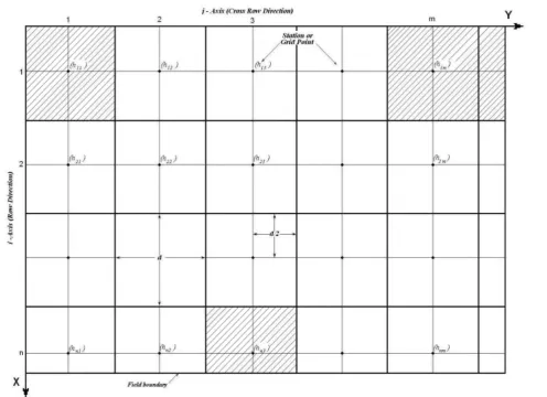
A field layout and the adopted coordinate system are shown in
Fig. 1. The grid elevations, hij (i=1,2,3…,nj in row direction
and j=1,2,3…,mi in cross row direction) were taken at equal
intervals (d). The numbers of rows and cross rows may not be equal. In this case, the stations (grid points) are form a matrix that has mxn dimensions. There was distance of half a square length between a grid point and land borders (Fig. 1). Thus, each station or grid point represented square shaped land with a side length of d. However, the area represented by each grid point was not always square shaped. Sometimes this area may be bigger or smaller than one unit of square. The area
represented by any station (Fij), was the area formed by
connecting the side midpoints of the station and adjacent
stations. For instance, grid points such as h11, h21, h23, h32
represented the areas of 1.0 unit, h1m, h2m, h3m grid points
represented areas bigger than 1.0 unit and grid point like hn1,
hn2, hnm represented areas smaller than 1.0 unit (Ayranci and
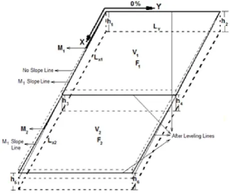
Temizel, 2011). Similarly; there is a somewhat different application for the application of variable sloped land grading in one direction. As a characteristic of the method, in the application of variable sloped grading in one direction, the
surface has to be leveled having two different slopes (Mx1,
Mx2) through the direction of water flow and on the opposite
direction the land has a surface no slope (Figure 2). For this reason, the amount of unit area represented by each grid point needs to be determined according to the lengths of the land
portions having different slope (Lx1, Lx2).
In the CAD program, contours were drawn with required intervals as coordinates and elevation values were entered for each grid and land borders were taken into consideration. Then, areas between every contour within the land borders were calculated one by one with the help of the program.
Fig 2. Schematic view of the land after grading
Before-Grading Volume
The principle of the method is based on to calculate the soil volume above a specific reference plane and the utilization of this soil volume during grading process. For the calculating the soil volume before grading, firstly the contour lines are passed over the land. Soil volumes between two consecutive contour lines are calculated separately, and at the end these volumes are summed up to determine the soil volume before grading. The equation below is used to calculate the volume of soil between two consecutive contour lines (Ayranci and Temizel, 2011).
= . ……….…. (1)
where; Vz; the volume of the soil between two consecutive
contour lines (m3), cz; the elevation of the smaller one of the
two consecutive contour lines (m), cz+1; the elevation of the
bigger one of the two consecutive contour lines (m), Fz; the
projection area between the two consecutive contour lines
(m2). In every land, there were land fractions higher than the
biggest contour line and lower than the smallest contour line.
The calculation of soil volume (Vr) in these fields, the
elevation values of the contour lines and the border point of the land in that field can be used with the help of the Equation
1. The total soil volume before grading (Vbl) could be obtained
by summing all of the volumes between the two grading points. Hence, the total soil volume before grading could be found with the help of Equation 2.
Vbl= ∑ + ………... (2)
where; Vbl; total soil volume before grading (m3), n; the
number of land fractions separated by contour lines in the
field, Vr; soil volume belonging to the field outside of contour
lines (m3), z; the number of areas between contour lines
(z=1,2,3,…..,z)
Finding the heights of corner points after the grading of the land
One of the basic rules of land grading is “neither the soil is brought from another place to the land to be leveled nor the soil be taken away from the land to be leveled to another place. In accordance with this principle, the soil volume of before
grading (Vbl) must be equal (Vbl = Val) to the soil volume after
grading (Val). Variable sloped grading in one direction is a
method used to reduce deep seepage losses, especially in surface irrigation methods. For this purpose, the field is leveled with a larger slope after the irrigation canal, and then with a lower slope. The application of variable sloped grading is a method used to facilitate the application of the border irrigation method. For this reason, the position of the channel where the irrigation water is received will determine the direction (X or Y) in which the land grading will be applied.
Also; the slope values (M1, M2) to be used and the land lengths
(Lx1, Lx2) having these slope values should be determined. In
the case of grading of the land variable sloped in the X direction, some properties related to the area after grading will occur as in Fig 2. According to the Fig.2, the following equations can be written.
= + ……….. (3)
where; is the soil volume after grading (m3), is the soil
volume of high sloped section (m3), is the soil volume of
low sloped section (m3).
= + ≫ = . ; = . ………. (4)
where; is the projection area of the high sloped section (m2),
is the projection area of the low sloped section (m2), is
the length of through slope of the high sloped section (m), is the length of through slope of the low sloped section (m), is the length of the edge no slope of the land (m).
The and equations can be expressed as;
= . ; = . ……… (5)
where; h1, h2, h3, h4, h5, h6 are the elevations of the corner
points of the land after grading. Accordingly, the following equations can be written regarding the elevations of the corner points of the land after grading.
ℎ = ℎ ; ℎ = ℎ ; ℎ = ℎ ……….. (6)
The equations and Y are become;
= . If necessary simplifications are made;
= . ……….. (7)
= . If necessary simplifications are made;
= . ……….. (8)
The elevations of the (ℎ = ℎ ) and (ℎ = ℎ ) corner points
(ℎ = ℎ ) = ℎ − . ; (ℎ = ℎ ) = ℎ − . …..…. (9)
(ℎ = ℎ ) = ℎ − . ≫(ℎ = ℎ ) = ℎ − . − . ……..………… (10)
where; M1 is the slope of the high sloped section (%), M2 is
the slope of the low sloped section (%). If these equations are placed in Equations 7 and 8;
=
.
. ……….. (11)
=
.
( . . )
. ……….. (12)
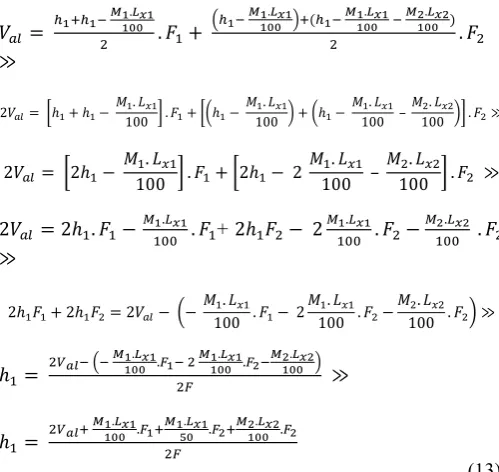
If these equations (11 and 12) are placed in Equation 3 and necessary simplifications are made;
=
.
. +
.
( . . )
. ≫
2 = ℎ + ℎ − .
100 . + ℎ − .
100 + ℎ − . 100 –
.
100 . ≫
2 = 2ℎ − .
100 . + 2ℎ − 2 . 100 –
.
100 . ≫
2 = 2ℎ . − . . + 2ℎ − 2 . . − . .
≫
2ℎ + 2ℎ = 2 − − .
100 . − 2 . 100 . −
.
100 . ≫
ℎ =
.
. . . .
≫
ℎ =
.
. . . . .
……… (13)
The height of the h1 point after grading is determined by
means of the Equation 13. If h1 = h2 according to equation 6,
the value of h2 point is also found. The Vbl value obtained from
equation 2 can be used instead of Val in the equation 13. After
finding the height of point h1 and h2 by the equation 13, the
height values of the point’s h3 - h4 and h5 - h6 are determined
with the help of the equations 9 and 10 respectively. Slope
values in the equation 13 are used with just numeric values, without sign.
Finding the heights of the grid points after grading
After finding the heights of the corner points, starting from h1
point, the elevation of the h1,1 grid point can be found with the
aid of equation 14.
ℎ , = ℎ −
.
……….... (14)
where; h1,1 is the height of the h1,1 grid, m, Lu is the edge
length of unit grid, m
Since the land has no slope in Y direction, the heights of the
grid points h1,2 , h1,3 and h1,4 will be equal to h1,1. The heights of
the following grid points in the X direction can also be found with the equation 15.
ℎ , = ℎ , − .
……….. (15)
Since the land has no slope in Y direction, the heights of the
grid points h2,2 , h2,3 and h2,4 will be equal to h2,1. Similarly, the
heights of the grid points h3,1 , h4,1 etc can be found by means
of equation 15. In this way, the heights of all the grid points on the ground are found. The cut and fill heights at the each grid point can be determined by comparing the grading grid heights with the natural grid heights. Depending on the cut or fill heights at each grid point, cut and fill volumes may be found at each grid unit. The volume of cut or fill at any station can be calculated by multiplying the cut or fill height of that station by the unit area value of the station.
, = ℎ, . . ……….. (17)
where; Vc,f is the volume of cut or fill in the grid unit, m3, hc,f is
the height of cut or fill in the grid point, m, Fu is the area of the
grid unit, m2, Cw is the area weighting factor.
Area weighting factor can be find by the equation below;
= . ……….. (18)
where; Lgx is the length of the edge which parallel to the X axis
of the area that the grid represents, m, Lgy is the length of the
edge which parallel to the Y axis of the area that the grid represents, m,
To reach the total cut and fill volume, the cut and fill volumes
in each station can be summed up. The cut/fill ratio (Rc/f) is
found by proportioning the total cut and total fill heights. At land grading, it is desired that the ratio of cut/fill according to the soil texture is between the values in Table 1. If the cut/fill ratio is within the desired limits, the grading process is performed according to the determined values.
Table 1. Cut/fill ratios according to the soil texture (Yıldırım, 2008)
Texture Kazı/Dolgu Oranı (Rc/f)
Sandy 1.15-1.25
Loamy 1.25-1.40
Loamy-Clay 1.40-1.60
Clay 1.50-1.80
If the cut/fill ratio is not within the range of the desired values, the height of the grading plane must be changed. In this case, the amount of change to be made at the height of the grading plane can be found by the following equation.
ℎ = / ………. (19)
where; hd is the amount of change to be made at the height of
the grading plane, cm, Vcf is the total cut and fill volume, m3,
Dc/f is the desired cut/fill ratio, Vc is the total cut volume,
m3, Vf is the total fill volume, m3, Fcf is the total projected area
Application of the method to a hypothetical area
In order to test the method, variable sloped grading calculations have been done on a hypothetical area. The
sample area is a size of 22100 m2 and a rectangular shape
having 170m in the X direction and 130m in the Y direction. The distance between grid points is 30m. Accordingly, the unit
grid area is 900 m2. Grading calculations has been done
assuming that the land has a sandy texture (the cut/fill ratio is
between 1.15 and 1.25) and for the slopes of M1(0.5%) and M2
(0.4%) through the X direction. It is assumed that the land
lengths (Lx1 and Lx2) with different slope values are equal
(85m).
The application of the method is carried out in the following stages. Firstly, as mentioned in the Section 2.1.1., the contour lines are passed on the land. After that, the grid points' locations and the amount of area represented by each grid point are determined. Depending, the soil volume before grading is determined. At this point, according to the method's characteristic (Section 2.1.2.), the soil volume after grading is
also determined. Subsequently, the height of corner point h1 is
determined by means of Equation 13. At this point, according
to Equation 6, the height of point h2 is also determined. By
means of Equations 14 and 15, the heights of all the grid points in the field can be determined. After determining the heights of the grid points, compared with the ground elevations in each grid point, the cut and fill heights and accordingly the cut and fill volumes in each grid are found by Equation 17.
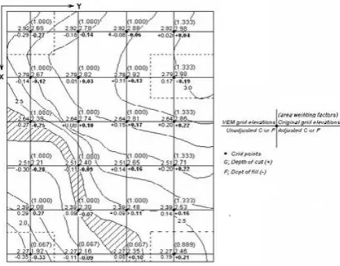
Figure 3. The grading results of the VEM for variable sloped grading in one direction
Table 2. The results of the variable sloped grading calculations of the VEM Method for slope values -0.5% (M1) and -0.4% (M2) in
the X direction
Attribute Results of VEM Method
Unbalanced ∑Volume of cut, m3 1705.3
∑ Volume of fill, m3 1819.6
Cut to fill ratio, Rc/f 0,937
Balanced ∑Volume of cut, m3 2015.8
∑ Volume of fill, m3 1579.6
Cut to fill ratio, Rc/f 1.276
Volume of cut per hectare, m3ha-1 911.7
Similarly, the cut and fill volumes at all grid points are found. The total cut volume is obtain by the cut volumes at each grid point are summed and the total fill volume is obtain by the fill
volumes at each grid point are summed. Rc/f is determined by
proportioning the total cut volume to the total fill volume. If
the Rc/f ratio is between the values given in Table 1, the grid
values found are accepted. If not, to bring it to the desired limits, the grading plane is replaced help of the Equation 18. Table 2 and Figure 3 are representing the results of the variable sloped grading in one direction of the Volume Equalization Method.
Conclusion
In this article; based on the Volume Equalization Method developed by Ayranci and Temizel 2011, variable sloped grading calculations in one direction are presented. The basis of the method is "the soil cannot be brought from the outside to the land grading area and the soil cannot be taken to the outside". Accordingly, the before and after grading soil volumes measured from a reference elevation are equal. In this study; it is given the mathematical principles of the method and it was applied to a hypothetical area with a size of 22100
m2 for testing the method for variable sloped grading in one
direction at rectangular fields. The presented method
eliminates the need for use trial and error procedures that existing land grading design methods involve to determine the planet hat balances cut and fill volumes. Although it is based on least-squares theory, it doesn’t have the time consuming calculations that appear in the conventional least-squares method. It is seen that both methods produced almost the same results in rectangular fields. As was done in the example application, the proposed method (VEM) can be performed manually using hand calculators. Its suitability to hand calculation is a big advantage. Furthermore, the design procedure can be easily translated to a computer or a calculator program. According to the unbalanced grading results (Table
2), the total cut volume was 1705.3 m3, and the total fill
volume was 1819.6 m3. The cut/fill ratio (Rc/f) was 0.937.
According to this conclusion, since the required cut/fill ratio according to soil properties should be in the range of 1.15-1.25, the grading plane had to be changed. After balancing process, it is necessary to increase the excavation height by 2 cm and the fill height by 2 cm. In this case, the total cut
volume is 2015.8 m3 and the total fill volume is 1579.6 m3.
And, The cut/fill ratio (Rc/f) is 1.276. This result can be
accepted. The cut volume per hectare for the newly developed
method is 911.7 m3. Because of the topography of the
hypothetical area is very rough, the values of the cut and fill volume are high.
REFERENCES
Ayranci, Y., K.E. Temizel, 2011. Volume equalization method for land grading design: Uniform sloped grading in one direction in rectangular fields, African Journal of
Biotechnology, 10 (21) pp. 4412-4419.
Bansal, C., G. Singh, D.K. Jain, and M. Kaur, 2014. Laser Land Leveling Prototype Development. International
Journal of Latest Research in Science and Technology, 3,
(6) pp. 130-134.
Brye, K.R., N.A. Slaton, and R. J. Norman, 2005. Penetration resistance as affected by shallow-cut land leveling and cropping, Soil & Tillage Research, 81, pp. 1–13.
Cazanescu, S., D. Mihai, R. Mudura, 2010. Modern technology for land levelling based on a 3D scanner.
Research Journal of Agricultural Science, 42 (3), pp.
471-478.
Chilur, R., P.S. Kamannavar, and Y.R. Manojkumar, 2016. Laser Land Levelling: It’s Impact on Slope Variation in Vertisols of Karnataka. Environment & Ecology, 34 (2A), pp. 740-744.
Dedrick, A.R., R.J. Gaddis, A.W. Clark, and A.W. Moore, 2007. Land Forming for Irrigation. In Design and
Operation of Farm Irrigation Systems, 2nd Edition (p.
320). American Society of Agricultural and Biological Engineers.
Demirtaș, Ç., and A.O. Demir, 2011. The use of least square method in land leveling projects on geographic information system (GIS). Uludag University, Journal of Agricultural
Faculty, 25 (1), pp. 27-40.
Jat, M.L., P. Chandna, R. Gupta, S.K. Sharma, and M.A. Gill, 2006. Lazer Land Leveling: A Precursor Technology for Resource Conservation). Rice-Wheat Consortium for the Indo-Gangetic Plains CG Block, National Agriculture Science Centre (NASC) Complex, DPS Marg, Pusa Campus, New Delhi 110 012, India.
Naresh, R.K., S.P. Singh, A:K. Misra, S.S. Tomar, P. Kumar, V. Kumar, and S. Kumar, 2014. Evaluation of the laser
leveled land leveling technology on crop yield and water use productivity in Western Uttar Pradesh. African Journal
of Agricultural Research, 9 (4), pp. 473-478.
Rickman, J.F., 2002. Manual for laser land leveling, Rice-Wheat Consortium Technical Bulletin Series 5. New Delhi-110 012, India: Rice-Wheat Consortium for the Indo-Gangetic Plains. p. 26.
Scallopi, E.J., and L.S. Willardson, 1986. Practical land grading based on least squares. J. Irrig. Drain. Eng., 112(2), pp. 98-109.
Sharifi, A., M. Gorji, H. Asadi, and A.A. Pourbabaee, 2014. Land leveling and changes in soil properties in paddy fields of Guilan province, Iran. Paddy Water Environ (2014) 12, pp. 139–145.
Shih, S.P., and G.J. Kriz, 1971. Symmetrical residuals methods for land forming design. Trans. ASAE. 14(6), pp. 1195-1200.
Yıldırım, O. 2008. Design of Irrigation Systems. Publication of Agricultural Faculty of Ankara University, No:518, Ankara University Printing house, p. 354, Ankara (In Turkish).
Zimmerman, K.R., A. Gross, M. O’Connor, G. Sapilewski, D.G. Lawrence, H.S. Cobb, L. Leckie, and P.Y. Montgomery, 2005. System and Method for Land Leveling, United States Patent No: US 6,880,643 B1, Apr. 19.