COMPARISON OF THE EQUIVALENT CIRCUIT MODEL AND THE TLM METHOD FOR FREQUENCY SELECTIVE SURFACE ANALYSIS

RESEARCH ARTICLE

COMPARISON OF THE EQUIVALENT CIRCUIT MODEL AND THE TLM METHOD FOR FREQUENCY

SELECTIVE SURFACE ANALYSIS

*,1

_{Dominic S. Nyitamen,}

_{Muhyaddin J.H. Rawa,}

_{Steve Greedy,}

_{Chris Smartt and}

2

_{David W.P. Thomas}

1

_{Electrical Electronic Engineering Department NDA, Kaduna- Nigeria}

2

_{George Green Institute for Electromagnetic Research, University of Nottingham, Nottingham, NG7 2RD, UK}

ARTICLE INFO

ABSTRACT

The Transmission line modeling method (TLM) and Equivalent circuit method are applied to the analysis of a dual band frequency selective surface (FSS) based on a double square loop design. The results are compared with experimental work. Results obtained from experiments conducted were then compared with those predicted by the numerical models. Good agreement between both numerical approaches and measurement has been demonstrated. The TLM results proved to be more accurate and robust, while the equivalent circuit method remained orders of magnitude faster

Copyright © 2015Dominic S. Nyitamen et al. This is an open access article distributed under the Creative Commons Attribution License, which permits unrestricted use, distribution, and reproduction in any medium, provided the original work is properly cited.

INTRODUCTION

Frequency selective surfaces (FSS) comprise a periodic array of patches or apertures in a conducting surface for frequency filtering. Many studies have been carried out on FSS due its

widespread applications (Parker et al., 1987; Lee and Langley,

1985; Jha et al., 2012). A wide range of geometrical

configurations of FSS structures have been modeled and the prediction of the reflection or transmission band achieved using various techniques. Three major numerical techniques used for the design and analyses of FSS are the modal analysis method, the equivalent circuit model and the spectral iteration

approach (Parker et al., 1991 and Mittra et al., 1988). In the

modal analysis method, the distribution of current induced in conducting elements (or fields in slots) is represented using a set of basis functions (usually sinusoidal functions or waveguide modes). Local fields are expanded as a set of Floquet modes (Marcuvitz, 1951). The sets of Floquet modes are then matched by applying standard electromagnetic boundary conditions to the conductors. A resulting integral equation involving the element currents is usually solved by the application of the method of moments (Munk, 2000) which generates a matrix equation for the coefficients of the current basis functions. This is a vector analysis and provides information on the polarisation of the scattered fields.

*Corresponding author:Dominic S. Nyitamen,

Electrical Electronic Engineering Department NDA, Kaduna- Nigeria.

The equivalent circuit approach models the arrays of elements in FSS as lumped impedances on a transmission line (Wu, 1995). This is a Quasi empirical equivalent circuits approach and is been employed (Hamdy and Parker, 1982) as design tools for quite complicated elements, requiring very little in the way of computing resources. In the Spectral Iteration technique, a first estimate of the element current induced by the incident field is used to calculate the local electric field distribution, which is then forced to zero at the surface of the conductors (Hamdy and Parker 1982). This modified field is in turn used to recalculate the element current distribution. The root mean square value of the ratio of the calculated field to the incident field over the conductors is used as an indicator of the progress of the iteration (Tsao and Mittra, 1982). In this paper, the predicted results obtained by two numerical methods, TLM and the equivalent circuit method are compared with the experimental measurements conducted on a double square loop band stop FSS. The two frequencies of interest in the double band stop FSS are 900MHz and 1.8GHz which correspond to the GSM900 and GSM1800 frequencies and are chosen because of their popularity and widespread use in mobile communications. The FSS realized can be used as wall paper for electromagnetic shielding in the two GSM bands in restricted rooms to prevent interference. The paper is organized as follows. Sections II and III introduce the TLM and equivalent circuit methods respectively. Section IV discusses the experimental setup and measurement carried out. Finally, section V presents discussions and conclusions.

ISSN: 0976-3376

Available Online at http://www.journalajst.com

ASIAN JOURNAL OF

SCIENCE AND TECHNOLOGY

Article History:

Received 01st _{February, 2015}

Received in revised form 13th _{March, 2015}

Accepted 19th _{April, 2015}

Published online 31st _{May, 2015}

Key words:

The TLM method

The TLM modeling technique applied in this work is based on a 3D time domain Electromagnetic field solver which allows the creation and solution of 3D electromagnetic problems on a structured cubic mesh (Christopoulos, 1995

numerical method is founded on the equivalence between voltages and currents on a transmission line network and electric and magnetic fields in 3D space.

transmission lines in the network allows the propagation of electromagnetic waves. The waves are character

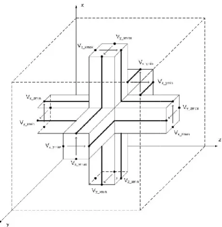
voltage and current and their associated Electric and Magnetic fields. The Electric and Magnetic fields are orthogonal to each other and to the direction of propagation. For example a z directed transmission line polarised in the x direction is associated with the fields Ex and Hy. The problem space is discretised into cubic cells where the cell size is significantly smaller than the shortest wavelength of interest in the analysis. Each cell face has two orthogonal TEM transmission lines (link lines) with associated Electric and Magnetic field components tangential to the cell face. The transmission lines incident from each face intersect at the cell centre forming a junction (Figure 1).

Figure 1. Symmetrical condensed node

The link transmission lines have distributed capacitance and inductance representing the permittivity and permeability of a vacuum. For materials other than free space, the permittivity or permeability may be augmented by the addition of suitably defined stub transmission lines. A voltage impulse incident on the cell centre junction from one of the link lines scatters back into the link lines, this process is described by a scattering matrix. The scattering matrix is defined such that the transmission line network models Maxwell's equations. The scattered voltage pulses reach the cell faces half a time later and connect to adjacent cells. The TLM algorithm can be considered as a discrete version of Huygen’s principle

(Christopoulos, 1995)

.

transmission line in the network (the simulation time

chosen to be the same. This property of the network provides discretisation in time and ensures time synchronisation of the The TLM modeling technique applied in this work is based on a 3D time domain Electromagnetic field solver which allows the creation and solution of 3D electromagnetic problems on a , 1995). This explicit is founded on the equivalence between voltages and currents on a transmission line network and d magnetic fields in 3D space. Each of the transmission lines in the network allows the propagation of electromagnetic waves. The waves are characterised by voltage and current and their associated Electric and Magnetic fields. The Electric and Magnetic fields are orthogonal to each other and to the direction of propagation. For example a z directed transmission line polarised in the x direction is The problem space is discretised into cubic cells where the cell size is significantly smaller than the shortest wavelength of interest in the analysis. Each cell face has two orthogonal TEM transmission lines ) with associated Electric and Magnetic field components tangential to the cell face. The transmission lines incident from each face intersect at the cell centre forming a

Figure 1. Symmetrical condensed node

lines have distributed capacitance and inductance representing the permittivity and permeability of a vacuum. For materials other than free space, the permittivity or permeability may be augmented by the addition of suitably A voltage impulse incident on the cell centre junction from one of the link lines scatters back into the link lines, this process is described by a scattering matrix. The scattering matrix is defined such that the l's equations. The scattered voltage pulses reach the cell faces half a time-step later and connect to adjacent cells. The TLM algorithm can be considered as a discrete version of Huygen’s principle The propagation delay on every nsmission line in the network (the simulation time-step) is operty of the network provides discretisation in time and ensures time synchronisation of the

scatter and connect processes in the network.

the cell is such that all 3 components of both electric and magnetic field are evaluated at the cell centre during the scattering process and tangential Electric

components are calculated half a time

faces during the connect process. Boundary conditions are applied on the outer surfaces of the problem space as required for the scenario under study. Boundary conditions may represent perfectly conducting surfaces or implement an absorbing boundary condition for example.

apply the open source TLM code GGI_TLM

(www.girhub.com/ggiemr/GGI_TLM/

the dual band FSS. The GGI_TLM code allows the

imposition of a ‘wrapping

(www.girhub.com/ggiemr/GGI_TLM

simulation of an infinite periodic array of elements with a model of a single cell of the FSS structure. The GG_TLM code simulates in the time domain method as opposed to frequency domain methods like method of moments (MOM). Frequency domain results are obtained by the Fourier Transform thus GGI_TLM predicts the response of the FSS over the entire frequency range of interest in a single simulation. Figure 2 shows the mesh generated for a u cell. The square loops are modeled as perfect electrical conductors. Wrapping boundary conditions are placed on the

x and y boundaries. An absorbing boundary condition is

imposed on the z boundaries to absorb the scattered field. In

the TLM model a pulse plane wave is launched towards the FSS sheet. Time domain fields are recorded on both the reflection and transmission side of the FSS until all the significant electromagnetic interactions have taken place.

Fig. 2 Mesh generated for unit cel

This is followed by a post processing procedure which involves Fourier transformation to obtain the reflection and transmission coefficient characteristic of the design at the desired frequencies. A TLM simulation of the FSS typically takes less than an hour on a single processor desktop PC. This should be compared with FSS simulation in frequency domain employing method of moments with the computational time reported as being 4 hours for a double square loop

al., 2009). In this paper a double s

block the GSM900 and GSM1800 frequencies is studied. The Fig.3 shows the relative spacing of elements of the double square loop FSS.

scatter and connect processes in the network. The structure of is such that all 3 components of both electric and magnetic field are evaluated at the cell centre during the scattering process and tangential Electric and Magnetic field components are calculated half a time-step later at the cell ct process. Boundary conditions are applied on the outer surfaces of the problem space as required for the scenario under study. Boundary conditions may represent perfectly conducting surfaces or implement an absorbing boundary condition for example. In this work we

apply the open source TLM code GGI_TLM

www.girhub.com/ggiemr/GGI_TLM/) to the modeling of The GGI_TLM code allows the

imposition of a ‘wrapping boundary condition’

www.girhub.com/ggiemr/GGI_TLM), allowing the

simulation of an infinite periodic array of elements with a model of a single cell of the FSS structure. The GG_TLM code simulates in the time domain method as opposed to ethods like method of moments (MOM). Frequency domain results are obtained by the Fourier Transform thus GGI_TLM predicts the response of the FSS over the entire frequency range of interest in a single Figure 2 shows the mesh generated for a unit FSS cell. The square loops are modeled as perfect electrical conductors. Wrapping boundary conditions are placed on the y boundaries. An absorbing boundary condition is z boundaries to absorb the scattered field. In l a pulse plane wave is launched towards the FSS sheet. Time domain fields are recorded on both the reflection and transmission side of the FSS until all the significant electromagnetic interactions have taken place.

Fig. 2 Mesh generated for unit cell

This is followed by a post processing procedure which involves Fourier transformation to obtain the reflection and transmission coefficient characteristic of the design at the desired frequencies. A TLM simulation of the FSS typically ur on a single processor desktop PC. This should be compared with FSS simulation in frequency domain employing method of moments with the computational time

reported as being 4 hours for a double square loop (Campos et

Fig.3. Double square loop elements

Equivalent Circuit Method

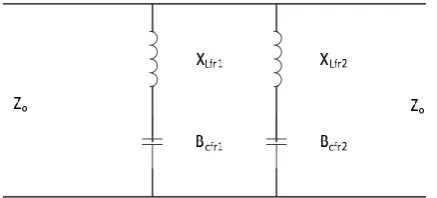
The equivalent circuit approach models the FSS as a network of lumped impedances on a transmission line (Munk, 2000). This method is not as precise as a full 3D simulation for frequency selective surface analysis however it is used as a quick method for estimating the characteristics of FSS structures. Each square of the FSS are modeled with inductor and capacitance in series. The resonance of outer square

comprise the inductance XLfr1and the capacitance Bcfr1, while

the second resonance has inductance XLfr2 with capacitance

Bcfr2.

Fig. 4. Circuit model of a dual band-stop FSS

Various geometrical structures of the FSS have been studied extensively using numerical and analytical methods including double-square-loop (Parker, 1991 and Mittra, 1988). The equivalent circuit method is applied to a dual band-stop FSS by first evaluating the expressions for the equivalent circuit

elements in Fig.4. XLfr1, XLfr2, BCfr1 and BCfr2 are the

inductances and the capacitances at the first and second resonant frequencies respectively. The normalized inductances and capacitances are given by the following equations (Marcuvitz, 1951):

where

λ

is the wavelength and

The function ( , , , ) for normalized capacitance is

solved by replacing ℎ and of the normalized

inductance. Equations above are appropriate for wavelengths

and incidence angles between the range p (1+ )/ < 1. It

can be used to predict the reflection and transmission of plane waves, TE and TM and it cannot be used in modeling cross-polarization (Lee and Langley, 1985).

The equivalent circuit has four reactive elements,

, , are calculated as follows [2 ],

[8]:

The factor F, which stands for the normalized inductances and capacitances of the strip grating for both TE and TM incidence were presented in (Munk, 2000). Using the above equations, it is possible to calculate the inductances and capacitances not only at normal incidence but also in the TE and TM planes. The transmission coefficient T of the array is determined from

|T|2 = 4/(4+|Y|2)

where Y is the admittance of the FSS equivalent circuit model. This transmission coefficient T is implemented with a Matlab code.

Measurements

The Double Square loop FSS shown in Fig. 5 was made by placing copper tape of paper substrate. The dimension of the inner square is 43mm by 43mm and a width of 7mm, while the outer square is 98mm by 98mm and

width 11mm. The sample FSS sheet consists of a 5 by 5 matrix as shown in Fig.5.

Fig. 5. FSS sheet

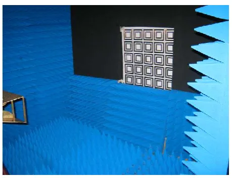
The FSS sheet is placed between the transmitting and receiving antennas in an anechoic chamber connected to a vector network analyzer as depicted in Fig.6. A photograph of the actual measurement is shown in figure 7.

Table 1 gives the parameters used in the equivalent circuit

model. Table 2 shows the resulting resonant frequencies, f1 and

f2 as well as the corresponding resonance values for TLM

simulation and measurements.

Table 1. Double Square Loop dimensions (m)

p d1 w1 g1 d2 w2 g2

0.11 0.096 0.010 0.014 0.060 0.007 0.008

Fig.7. S21 measurement setup in Anechoic Chamber

Fig. 8 shows a plot of the magnitude of the transmission coefficient versus frequency for the numerical methods

(Equivalent model and GG_TLM) together with

measurement.

Fig.8. S21 for Circuit Model, GG_TLM and Measurements

Overall there is reasonable agreement in the results between the numerical methods and measurements. The first

transmission band centered on f1 (900MHz) occurs at

approximately the same frequency for Circuit model, GG_TLM and measurements. We observe from the numerical method that this resonance is less dependent on the inner square side length than on its width. There is however some

difference seen in the frequency of the second resonance at f2

(~1.8GHz) between the circuit model and the GGI_TLM and measurement. This second resonance is determined mainly by the dimensions of the inner square.

Conclusion

In this paper the TLM modeling method and equivalent circuit model are compared in terms of accuracy and computational time in analyzing an FSS structure. The results are compared with measurements for a double square loop band stop FSS structure operating at 900MHz and 1.8GHz. The time domain TLM method has the advantage of providing results over a wide frequency band with a single simulation. This makes the process of simulation faster than 3D frequency domain methods such as the method of moments. The Equivalent circuit model remains the fastest in terms of computational time however the results are less accurate compared to TLM.

Fig. 6 Measurement Setup

f1 f2

Eqv. Cct Model

GG_ TLM

Exp’tal results

Eqv. Cct Model

GG_ TLM

Exp’tal results

REFERENCES

Parker, E. A. and R. J. Electronic Letters, 1987, 19(17),

675-677.

Lee, C. K. and R. J. Langley, “Equivalent circuit models for frequency selective surfaces at oblique angles of

incidence”. 1985 IEE Proc. H, 132, 395-399.

Jha, K.R. G. Singh and R. Jyoti “A simple synthesis technique of single-square-loop frequency selective surface” Progress in Electromagnetic Research B, 2012 Vol. 45, 165-185.

Parker, E.A. “The gentleman’s guide to frequency selective

surfaces” 17th Q.M.W. Antenna symposium, 1991,

London.

Mittra, R. C.H. Chan and T. Cwik, “techniques for analyzing Frequency Selective Surfaces – a review”, IEEE proceedings, 1988, 76(12), 1953 – 1616

Marcuvitz, Microwave Handbook Editors McGraw-Hill, Nova

Iorque, 1951

Munk B.A. Frequency Selective Surfaces Theory and Design

Wiley-Interscience Publication John Welley & Sons, Inc. Canada 2000.

Wu T.K. Frequency selective surface and grid array, John

Wiley and Sons, Nova York, E.U.A., 1995

Campos, A.L.P.S R.C.O. Cesar, and J.I.A. Trindade “A comparison between the equivalent circuit model and moment method to analyze FSS “International Microwave and Optoelectronics Conference” 2009, pp. 760-765 Hamdy, S. M. A. and E. A. Parker, “Current distribution on

the elements of a square loop frequency selective

surface”, Electron. Lett.. 1982, 18, pp. 624-626

Tsao, C. H. and R. Mittra. “Spectral iteration approach for analyzing scattering from frequency selective surfaces”. IEEE Trans. on Antennas and Propagation, 1982, 30, 303-308.

*******