Statistics-Based Matching Cost Function for Intensity Transformation

Statistics-Based Matching Cost Function for Intensity

Transformation

Phuc Nguyen Hong, Chang Wook Ahn

*

Department of Computer Engineering, College of Information & Communication Engineering, 2066 Seobu-ro, Jangan-gu, Suwon, Gyeonggi-do 440-746, Republic of Korea.

* Corresponding author. Tel.: +82312994677; email: [email protected] Manuscript submitted October 30, 2015; accepted April 18, 2016. doi: 10.17706/ijcce.2016.5.6.455-464

Abstract: Stereo matching is a challenging task due to stereo images being affected by many factors such as radiometric distortion, sun and rain flare, flying snow, occlusion and object boundaries. However, most of the existing stereo matching methods assume that corresponding pixels in left and right images have the same intensity; accordingly, the stereo matching methods use simple matching cost functions. As a result, they degrade their performance significantly when operating with real-world stereo images whose intensities of corresponding pixels can be arbitrarily transformed. State-of-the-art matching cost functions under conditions of distorted intensities between stereo images, such as the census transform, adaptive normalized cross-correlation, and the support local binary pattern perform with limited accuracy. In this paper, we propose a novel matching cost function based on a robust order statistic coefficient and segmentation that can operate accurately under various conditions of transformed intensities between stereo images. Based on the robust order statistic coefficient, the proposed matching cost function can tolerate local, monotonically nonlinear changes in intensities between the left and right images. By using the information of segmentation, the matching cost function operates accurately at object boundaries. The qualitative and quantitative experimental results obtained using stereo images in different datasets under various conditions show that our proposed matching cost function outperforms state-of-the-art matching cost functions in indoor and outdoor stereo images with various radiometric distortions.

Key words: Matching cost, order statistics, stereo matching.

1.

Introduction

Stereo matching aims to find the depth for each pixel in the left image (e.g., using the left image as a reference image) of a stereo pair of images. It is still studied intensively because of its vital applications such as interactive robot navigation, self-driving cars, view interpolation, and three-dimensional reconstruction [1], [2]. According to Scharstein et al. [3], most of the stereo matching methods perform four steps: the matching cost computation, cost aggregation, disparity computation/optimization, and disparity refinement processes. Each step is important for achieving a high-quality disparity map, where the matching cost computation is a basic and important step that significantly affects the accuracy of the disparity map.

so their performances are degraded severely in real stereo images whose intensities are arbitrarily changed [8].

Local stereo matching methods typically consist of matching cost computation, cost aggregation, disparity computation, and disparity refinement steps, such as [9]-[13]. Clearly, matching cost computation is compulsory for all stereo matching methods, so the performance of a stereo matching method heavily relies on the accuracy and robustness of the matching cost function used. A matching cost function computes a matching cost value for each pixel, p, in the left image with a disparity hypothesis, d, to create a matching cost image space, C, in which Cd(p) is a matching cost value for p and d. From C, we can obtain a

disparity value for p as follows:

 

arg min



_d

 



d

D p



C

p

(1)

where D is a disparity map.

The contributions of our work are as follows. First, we show that although the order statistics coefficient (OSC) is a good measure for computing the correlation between two sets of data points, it is not applicable to stereo matching as a matching cost function. This is due to the OSC becoming undefined when all data points have equal values. We propose an ROSC, which can overcome the weakness of the OSC while keeping the important properties of OSC. Second, we propose a matching cost function using segmentation and an ROSC, abbreviated SROSC. As a result, the proposed matching cost function addresses the fattening effect and radiometric distortion problems in stereo matching. Finally, we conduct experiments to evaluate the proposed matching cost function and compare it with state-of-the-art matching cost functions using stereo images captured with radiometric distortion from different datasets. Experimental results show that the proposed matching outperforms the state-of-the-art matching cost functions in different datasets.

1.1.

OSC

The OSC, which was proposed in [14], can measure the monotonically non-liner association of two sets of data points using order statistics and the rearrangement inequality [15]. The OSC works on the principle that two sets of data points are highly correlated if large (small) values of one set are associated with small (large) values of another set.

Consider X 



x x₁, ₂, ,x_m



and Y 



y y₁, ₂, ,y_m



, two time series of length m. Forming the two time

series pairwise results in a set,

Z





z z

₁

,

₂

,

,

z

_m



, where

z

_i





x y

_i

,

_i



. Rearranging Z according to the

values of

x

_i, we get a new ordered set





1 2

 

1 2





1 1, 1 , , 1, m

Z  x y x y , where



x₁1 x1_m



are called the

order statistics of

X

, and

y

₁2

,

,

y

_m2 are the associated concomitants [16], [17]. On the other hand,

rearranging Z according to the values of

y

i , we obtain a set,





 





2 1 2 1

2 1

,

m

,

m

,

m

Z



x y

x

y

, where

1 1

1 m

y





y

. The OSC is defined as follows:









1 1 2

1 1

1 1 1

1 1

( , )

m

i m i i

i m

i m i i

i

l

l

r

OSC L R

l

l

r

     











(2)

1.2.

Motivation to Improve OSC

The OSC is highly sensitive to changes in association, tolerates monotone nonlinear transformations, and is robust to noise [14]. This makes the OSC suitable to use as a metric for measuring the image similarity.

Given two image regions of the same size, set Z can be constructed from the two image regions and the OSC

value can be computed using Z to measure the relationship between the image regions. An OSC value represents the degree of correlation between the two regions.

We denote

d



[ 0]

d

T for the disparity hypothesis, and [ ]T

p xy for a pixel in the left image; the

corresponding pixel in the right image is '

p  p d. Let L_{( )p} and R(p) be two pixel windows of the same

size, m. For the sake of simplicity, we denote

L

and

R

by

L

_{( )p} and

R

(p) , respectively. For

window-based matching cost functions in stereo matching, for each pixel p, in the left image, a window of

pixels,

L

_{( )p} , centered at p is exploited to compute the matching value. Accordingly, the number, d, of candidate windows,

R

_(p), in the right image is constructed and then each of the candidate windows is

measured for the degree of image similarity. The OSC can be used to measure the degree of similarity between pairs of pixel windows (one window from the left image and one window from the set of candidate windows from the right image). A larger OSC value of a window pair indicates more correlation (image similarity) between them. An OSC-based matching cost function can tolerate local, monotonically nonlinear intensity transformation between pair of pixel windows. This is a very important property for a matching cost function because stereo images in real-world situations are affected by many factors and their intensities can be arbitrarily transformed such as globally/locally linear/non-linear intensity changes.

However, a problem preventing the OSC from being applicable to stereo matching is that the OSC is undefined for a pixel window whose pixels have equal intensities. Pixels from severely textureless image regions or from images captured under illumination and exposure configurations that are too large/small are likely have the same intensity. Furthermore, road-driving images often contain homogenous intensity regions such as walls, the sky, and sun flare-affected regions. To illustrate this, we use some images from the Middlebury and Kitti datasets, and compute their textureless map in which a pixel is considered textureless if the variance of its corresponding pixel window is zero (all pixels over its window have the same intensity).

1.3.

ROSC

The idea of an ROSC is that we monotonically increase the value of each element in ordered sets

Z

₁ and

2

Z

by its rank in

Z

₁ and

Z

₂. Similar to the OSC, an ROSC forms the two time series pairwise first, resulting in a set,

Z

₁





z z

₁

,

₂

,

,

z

_m



, and rearranges

Z

according to the values of and

y

_i to result in

new ordered sets,









1 2





1 1

,

12

,

,

m

,

m

Z



x y

x

y

and

Z

₂







x y

₁

,

₁₂



,

,



x

1_m

,

y

_m2





, respectively. After

this, increasing the value of each element in

Z

₁ obtains a new set, '





1' 2'

 

1' 2'





1 1

,

1

,...,

m

,

m

Z



x

y

x

y

, where

 

1' 1 1

i i i

x



x



x

and

y

_i2'



y

_i2



 

y

_i2 . Similarly, multiplying each element in

Z

₂ by its rank in ordered set

2

Z

obtains a new set, '





2' 1'

 

2' 1'





2 1

,

1

,...,

m

,

m

Z



x

y

x

y

, where

y

_i1'



y

1_i



 

y

1_i is the rank of element 1

i

x

in

the sorted set

Z

₁, and

 

1 i

x



and

 

2

i

y



are the ranks of elements 1

i









1' 1' 2'

1 1

1' 1' 1'

1 1

( , )

m

i m i i

i m

i m i i

i

x

x

y

ROSC X Y

x

x

y

     











(3)

Here, by exploiting the sorted sets, Z1 and Z2, the ranks of and

y

_i1, can be computed as

x

1_i =

i

and 1

i

y



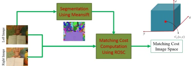
. An ROSC has several properties as follows.

Fig. 1. Flow chart of the proposed matching cost function.

Property 1: An ROSC is within the interval [-1, 1]. Proof. According to [18], rearrangement follows.

1' 1' 1' 2' 1' 1'

1

1 1 1

m m m

m i i i i i i

i i i

x

_{ }

y

x y

x y

  











(4)

and

1' 1' 1' 2' 1' 1'

1 1

1 1 1

m m m

m i i m i i i i

i i i

x

_{ }

y

x

_{ }

y

x y

  











(5)

Subtracting (4) by (5) and dividing the difference by



1' 1'



1'

1 1

m

i m i i

i

x

x

_{ }

y







. We have

 

1

ROSC x y

 

,



1

,

which completes the proof Property 2:



,



1( 1)

ROSC X Y

  

when

X

and

Y

_{have a monotonic decreasing (increasing) relationship.}

Proof. Assuming

y

_i





 

x

_i if

y

_i





 

.

is a decreasing function we have 2' 1' 1

i m i

y



y

  for all i.

Subtituting this into Eq.(3), We have

ROSC X Y



,



 

1

. Similarly, if



 

.

is an increasing function, it

results in 2' 1'

i i

y



y

for all i and eventually

ROSC X Y



,





1

Performing robustly with stereo images captured under different conditions is crucial to a matching cost function due to real-world stereo images being affected by many factors. Like Census, an ROSC, when applied to stereo matching as a matching cost function, can tolerate local, monotonically nonlinear intensity transform between stereo images; therefore, an ROSC-based matching cost function has good potential to operate well in stereo images taken in various situations. From the inherent benefits of an ROSC, we deeply investigate an ROSC-based matching cost function in the context of stereo matching and propose a matching cost function that combines an ROSC and segmentation. In the proposed matching cost function, segmentation is exploited to use pixels that locates in the same segmented regions. To do this, we use a common assumption in stereo matching that states that pixels having similar pixel intensities are very likely to be in the same image structure, and have similar disparities. This assumption is exploited in [5] to reduce the fattening effect. Fig. 1 shows the flowchart of the proposed matching cost function. In our work, we use the mean-sift algorithm [16] to segment the left image of a stereo pair.

In window-based matching cost functions, a window size with radius r _{is required to determine a set of}

pixel neighbors for each pixel, p. The coordinates of the given window, w, are computed as follows.







_w

,

_w

|

_{q q}



W



x

y

 

r

x

   

r

r

y



r

(6)

Let

I

_and

I

1 _{be the left and right images. In the proposed cost function, the coordinate of}

L

_p for

pixel p is determined as follows.



|

,

,



p q w p q w p

L



q q



I x



x



x y



y



y

(7)

Similarly, the coordinate of

R

_p' for pixel

p

'

in the right image,

I

'

is determined as follows





'

' | '

,

'

,

'

p q w p q w p

R



q q



I x



x



x



d y



y



y

(8)

In our work, we use the information of segmented image regions to determine if two pixels are in the

same segmented region. Let

N

p and

N

p' be a set of pixel neighbors for

p

and

1

p

, respectively, and

p

_{be the index of a segmented region in the segmented left image contains}

p

The two sets,

N

_pand

N

_p', are determined as follows:







|

,

,

1



p p

N



q q



L



p q



(9)

And



' ' 1



' ,

|

,

p p p

N



q q



R

q



N q

 

q d

(10)

where



 

p q

,

is the indicator function which determines if the two pixels, p and q, are in a segmented



,



1

if

0

otherwise

p

q

p q









_





(11)

Once

L

_p and

R

p' are determined, a matching cost value at pixel

p

in the left image and a disparity

hypothesis,

d

is computed as follows:



'



1

,

( )

2

p p

d

ROSC L R

C

p





(12)

An SROSC matching cost value is in interval [0, 1]. A smaller value of an SROSC indicates a higher degree of similarity between

N

_pand

N

_p'.

2.

Experimental Results

We conducted experiments to investigate the proposed matching cost function using the Middlebury dataset and compared it with state-of-the-art matching cost functions including the ANCC, Census, ADCensus, and SLBP. We used the available source code of the ANCC in [17]. We set the window size to be the same (11× 11) for the test matching cost functions. For the other parameters of the ANCC and ADCensus, we used the same values as the original papers, [5] and [18]. For SROSC, we used the mean-sift algorithm [19] to segment the left images of stereo pairs. The mean-sift segmentation parameters for the color bandwidth, spatial bandwidth, and minimum number size are 5, 4, and 20, respectively. All of the matching cost functions in this paper are evaluated using the average percentage of erroneous pixels in all zones, except occlusions, from disparity maps obtained using Eq. (1) and are computed at an error threshold of 1 pixel.

2.1.

Middlebury Dataset

To measure the strengths of the test matching cost functions in stereo images with radiometrical distortion, we used the Middlebury dataset [20], which contains stereo pairs captured under different lighting and exposures. The illuminations are indexed as 1, 2 and 3, and the exposures are indexed as 0, 1 and 2 with the available disparity ground truth. For simplicity, we used [I2E1/I2E2] as the abbreviation for a pair of stereo images for which the left image is with illumination 2 and exposure 1 (I2E1) and the right image is with illumination 2 and exposure 2 (I2E2). We fixed the left image to I2E1, while the right image changed with the eight remaining different conditions: I1E0, I1E1, I1E2, I2E0, I2E2, I3E0, I3E1, and I3E2. Stereo images with different exposures are global intensity transformations, whereas those with different illuminations are local changes of intensities.

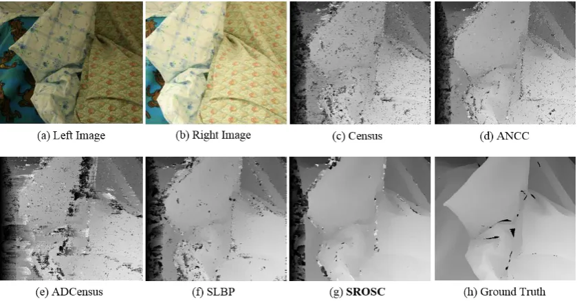
Fig. 2 shows the results of the test matching cost functions under different exposure settings. Fig. 2(a) shows left images with I2E1, and Fig. 2(b) shows right images with I2E2. The disparity maps of Census, the ANCC, ADCensus, SLBP, and SROSC are shown in Fig. 2(c)-Fig. 2(g), respectively. Fig. 2(h) shows the ground truth of the left image.

The reason for this occurring in Census is that it encodes local structures and produces bit strings by comparing the intensity of an anchor pixel with that of its neighbors. Census encodes a pixel pair in a binary value that represents a relative order; this causes the Census encoding to be ambiguous in textureless image regionsin which relative order of pixel pair more likely change under radiometrical distortions. In cases in which anchor pixels are intensity-transformed, the encoding output of Census is significantly affected. The ADCensus disparity maps are visually more erroneous than the Census ones due to stereo images with radiometric distortion; the AD had a negative effect in ADCensus.

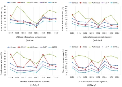
Fig. 3. Quantitative comparisons of the test matching cost functions using a winner-takes all strategy with Middlebury stereo image pairs with varying illumination and exposure configurations. (a) Aloe. (b) Baby1.

The ANCC relies on the color of an anchor pixel to compute a weight for each pixel in a window. When the colors of anchor pixels are radiometrically distorted or different largely from the colors of their neighbors, this leads to weights being largely changed. In addition, the ANCC’s assumption of a Lambertian reflectance object likely does not hold under radiometric distortions between stereo images. The disparity maps produced by SLBP reduce errors more compared to Census due to its use of more constraints on the relative orders among pixels. In contrast, as a result of SROSC using more pixels and being sensitive to the degree of a relative order, the SROSC disparity maps look more accurate than the SLBP ones. Overall, the disparity maps produced by SROSC are more accurate than those of ADCensus, Census, the ANCC, and SLBP.

Fig. 3 shows the quantitative comparison of the test matching cost functions using the different Middlebury sub-datasets. In this figure, I1E0 denotes the right image with illumination 1 and exposure 0. Census and the ANCC are comparable in different sub-datasets. For each sub-dataset, the ANCC and ADCensus displayed more fluctuation with different illumination and exposure settings than Census, SLBP, and SROSC due to the ANCC exploiting pixel colors to compute weights and ADCensus incorporating the AD that uses the color-consistent assumption. Census, SLBP, and SROSC were more stable as a result of them being based on the relative orders of pixels for computing their matching values; therefore, they can operate accurately and the order of pixels is preserved. SROSC had the most robust and accurate performance in all of the test sub-datasets. In a sub-dataset, the test matching cost functions performed differently for different illumination and exposure configurations, and SROSC was generally superior to the other test matching cost functions.

2.2.

Time Complexity

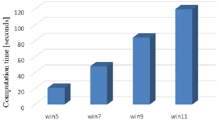
To measure the computation time of the proposed data cost, we used the Aloe images with a resolution of 427×370 and a disparity range of 70. We only measure the computation time required to compute its matching cost image space. Our test platform is a PC equipped with Intel core i7, a 4.00 GHz CPU, and 8.00 GB of memory. Fig. 4 shows the computation times required to compute the disparity image space of the proposed matching cost method with different window sizes. In Fig. 4, win5 indicates that SROSC uses a window size of 5×5. SROSC, with an 11×11 window size, took about 122 seconds to compute the matching cost image space, whereas SROSC, with a 5×5 window size, only needed about 21 seconds.

Fig. 4. Computation time.

3.

Conclusion

and the experimental results show that the proposed matching cost method was superior to the state-of-the-art matching cost methods across the datasets.

A robust order statistics coefficient can tolerate a monotone transformation of data points. In this paper, a robust order statistics coefficient is applied in stereo matching as a matching cost function. However, a robust order statistics coefficient can be used for image similarity; therefore, applying it in other computer vision applications such as template matching, texture classification, and optical flow is our future work.

Acknowledgment

This research was supported by Basic Science Research Program through the National Research Foundation of Korea (NRF) funded by the Ministry of Science, ICT & Future Planning (NRF-2015R1D1A1A02062017).

References

[1] Trucco, E., & Verri, A. (1998). Introductory Techniques for 3-D Computer Vision. Prentice Hall PTR. [2] Cyganek, B., & Siebert, J. P. (2009). Introduction to 3D Computer Vision Techniques and Algorithms. Wiley. [3] Scharstein, D., & Szeliski, R. (2002). A taxonomy and evaluation of dense two-frame stereo

correspondence algorithms. Intl. J. Comput. Vis., 47(1-3), 7-42.

[4] Hirschmuller, H., & Scharstein, D. (2009). Evaluation of stereo matching costs on images with radiometric differences. IEEE Trans. Pattern Anal. Mach. Intell., 31(9), 1582-1599.

[5] Heo, Y. S., Lee, K. M., & Lee, S. U. (2011). Robust stereo matching using adaptive normalized cross-correlation. IEEE Transactions on Pattern Analysis and Machine Intelligence, 33, 807-822.

[6] Nguyen, V. D., Nguyen, D. D., Nguyen, T. T., Dinh, V. Q., & Jeon, J. W. (2013). Support local pattern and its

application to disparity improvement and texture classification. IEEE Trans. on Circuits and Systems for

Video Technology.

[7] Dinh, V. Q., Nguyen, V. D., & Jeon, J. W. (2015). Robust matching cost function for stereo correspondence

using matching by tone mapping and adaptive orthogonal integral image. IEEE Transactions on Image

Processing, 24(12).

[8] Hirschmuller, H., & Scharstein, D. (2007). Evaluation of cost functions for stereo matching. Proceedings of Conference on Computer Vision and Pattern Recognition.

[9] Hong, P. N., Ali, M., & Ahn, C. W. (2014). Robust stereo matching method for radiometric distortion

between images. International Journal of Computer and Electrical Engineering.

[10] Nguyen, H. P., Tran, T. D., & Dinh, Q. V. (2012). Local Stereo Matching by Joining Shiftable Window and Non-Parametric Transform. Springer-Verlag Berlin Heidelberg, 133-142.

[11] Hong, P. N., & Ahn, C. W. (June 2014). Stereo matching using fusion of spatial weight variable window and adaptive support weight. International Journal of Computer and Electrical Engineering, 6(3).

[12] Tran, T. D., Nguyen, H. P., & Dinh, Q. V. (2012). Stereo Matching by Fusion of Local Methods and Spatial Weighted Window. Springer-Verlag Berlin Heidelberg, 167-175.

[13] Nguyen, P. H., Thi, D. T., & Dinh, V. Q. (2012). Enhancement of local methods by using spatial support

weight. Proceedings of 2012 IEEE International Symposium on Signal Processing and Information

Technology (pp. 245-250).

[14] Xu, W., Chang, C., Hung, Y. S., Kwan, S. K., & Fung, P. C. W. (2007). Order statistics correlation coefficient as a novel association measurement with applications to biosignal analysis. IEEE Trans. Sig. Proc., 55, 5552-5563.

[16] Mitrinovic, D. S., Pecaric, J. E., & Fink, A. M. (1993). Classical and New Inequalities in Analysis. Kluwer Academic, Dordrecht.

[17] ANCC and MIS source codes. From http://cv.snu.ac.kr/softwares

[18] Mei, X., Sun, X., Zhou, M., Jiao, S., Wang, H., & Zhang, X. (2011). On building an accurate stereo matching

system on graphics hardware. Proceedings of GPUCV.

[19] Comaniciu, D., & Meer, P. (2002). Mean shift: A robust approach toward feature space analysis. IEEE Transactions on Pattern Analysis and Machine Intelligence.

[20] Middlebury dataset. From http://vision.middlebury.edu/stereo/data/

Phuc Nguyen Hong received the B.S in science service from Auckland University of Technology (AUT), New Zealand in 2013. She is currently working toward the combine master and PhD degrees at the Computer Engineering Department, Sungkyunkwan University, Suwon, Republic of Korea.

Her research interests include genetic algorithms and computer vision.

Change Wook Ahn received the PhD degree at the Department of Information and Communications, Kwang-Ju Institute of Science and Technology, Kwang-ju, Republic of Korea.

From 2007 to 2008, he was a research professor in Gwangju Institute of Science & Technology (GIST). He is currently an assistant professor in Sungkyunkwan University (SKKU), Republic of Korea.