Scheduling Tasks to Minimize the Total
Computation and Communication Makespan
Teofilo F. Gonzalez
Department of Computer Science, University of California, Santa Barbara, CA USA 93106 Email: [email protected]
---ABSTRACT--- We study the problem of scheduling tasks in a distributed system where the data (and code) for a program may reside on a processor different from the one where it will be executed. The scheduling of the tasks is more complex than classical ones as one must not only take into consideration the processing times but also communication times. We present an off-line polynomial time approximation algorithm for the case when the processors can be partitioned into storage (client) and processing (server) nodes. Our algorithm is the first constant ratio approximation algorithm for this problem. Then we discuss generalizations of our problem, including an on-line distributed version, as well as versions that allow tasks to access multiple input files and generate multiple output files that reside in one or more nodes.
Keywords –Approximation Algorithms, Dual Objective Functions, Minimize Makespan, Scheduling.
--- --- Date of Submission: September 13, 2011 Revised: November 22, 2011 Date of Acceptance: November 26, 2011 ---
1.INTRODUCTION
S
cheduling problems arising from several research areas have been studied for more than five decades. The initial work was in operations research, computer science, and applied mathematics. More recently scheduling has been studied in the context of parallel, cluster, and grid computing. Our model falls under the broad umbrella of scheduling data-intensive distributed applications as well as ``cloud computing'' scheduling, i.e., where storage and processing of a task will be somewhere in the cloud. In this paper we discuss the problem of scheduling in distributed systems where the data (and code) for a program might not reside on the node where the task is to be processed. This scheduling problem is more complex than traditional ones. The complexity arises because in addition to balancing the processing workload, we also need to balance the time required to transmit the data (and code) needed by the programs. Algorithms for problems related to our problem appear in Refs. [1, 2, 3, 4, 5, 6, 7, 8]. This papers present heuristic and metaheuristics to generate sub-optimal solutions for different variations of our problem and present the results of an experimental evaluation of the performance of their algorithms. None of these algorithms have been shown to always generate schedules with a makespan that to be within a fixed percentage of the optimal one. On the other hand, our analysis is theoretical. We show that our algorithm is the first constant ratio approximation algorithm for our scheduling problem, i.e. the schedules generated have a makespan that is guaranteed to be withina given fixed percentage, independent of any problem parameters, of the optimal one.The system (``cloud'') consists of a set ofM nodes denoted by 1, f2, …, m. Each node j consists of mj identical processing elements (processors). Forexample,a node may be a parallel processor system, a cluster of computers,or a single computer with one or more cores.There are n independent tasks denoted by 1, 2, …, n to be processed. Processing task i by any processing element (processor) takes ti units of time,since all the processing elements are assumed to have the same processing capability.
The data (and code) for each task i is initially located at node si and, depending on the number of processing elements at the nodes and the total demand on the system, the task may or may not end up being scheduled for execution by a processor at node si. If task i is processed at another node, then the data1 required by the task needs to be transmitted from node si to the node where task i is to be processed. The transmission time is di time units. All of the task's data must be available at the processing node before any of its processors can begin executing the task. The data communication between nodes is performed through a channel in the communication network N. Node j has cjbi-directional channels. The bi-directional channelsare labeledin-channels and out-channels with respect to node i when the channels are used to bringin data or send out data, respectively. We assume that any one-to-one interconnection between nodes through the channels is supported by the communication network, and the routing to achieve the data interchanges can be computed in polynomial time. These assumptions are not too restrictive as a large number of interconnection networks satisfy these properties. We do not include this
1 Hereafter we use ``data'' needed by a task to refer to the ``data and
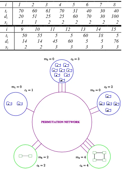
time in our analysis as it depends on the communication network. Once we determine that task i is to be processed by a processor at node j, we need to specify the out-channel to be used at node si, the in-channel to be used at node j, and the time interval when the data for task i is transmitted from node si to node j. Of course, the restriction is that the data from two or more tasks cannot be transferred using the same in-channel or the same out-channel at the same time. The objective function is to construct a minimum makespan computation schedule for the tasks that depends on the communication schedule constructed for the data communications. Fig. 1 depicts a simple problem instance defined over five nodes. This problem instance is fully specified in our example.
In this paper we consider the bipartite version of the problem when the set of nodes is partitioned into two sets called: Storage (Client) and Processing (Server) nodes. The data needed by the tasks is stored at the storage nodes and the processing of the tasks is to be performed at the processing nodes. To simplify the notation, assume that the first w nodes (1, 2, …, w) are the storage nodes, and the remaining ones (w+1, w+2,…, m) are the processing nodes. It is assumed that the number of channels, cj, for each of the processor nodes is equal to the number of processors at node nj. A 1-1 correspondence between processors and channels at each processing node is established2. For the storage nodes,
ci> 1.
Example
There are five nodes (m=5) and w=3. Nodes 1 – 3 store data for the tasks and nodes 4 and 5 process the tasks. The number of processors (mi) and number of channels (ci) at each node are given in Table 1. There are fifteen tasks (n=15). The processing time (ti), communication time (di) and the index of the node (si) where the data resides for each task is given in Table 2.
Given a set of independent tasks, their location and data requirements, our problem is to find the node, processor, and time at which each task is to be executed, as well as the (in- and out-) channels and time where the data (file) required by each task is to be transmitted. Our algorithms attempt to balance as much as possible the processing and communication times. We establish bounds between the balance in our schedules and the best possible communication and processing balance.
In this section, we discuss some well-known scheduling problems and their algorithms that our proposed algorithm invokes as sub-procedures (Sections 2.1 and 2.2), and we define and discuss the d-component vector scheduling problem as well as a new approximation algorithm, for d=2, that generates provably good solutions (Section 2.3).
2 This assumption simplifies the communication model. The number
of channels may be different than the number of processors. However, such systems are equivalent to our model by using virtual channels. The resulting problem is a generalization of our problem and for brevity it will not be discussed further.
This approximation algorithm is a central component of the scheduling algorithm proposed in this paper. Our scheduling algorithm is discussed in Section 3. In Section 4we discuss generalized versions of our problem. These versions allow the input data files to reside in multiple storage nodes and the tasks generate output files to be stored in one or more storage nodes.
Table 1: Number of Processors (mi) and Number of Channels (ci) for each Node in our Example.
i 1 2 3 4 5
mi 0 0 0 4 2
ci 1 3 2 4 2
Table 2: Processing and Communication Times, and Index of the Node where the Data for each Task Resides for all
the Tasks in our Example.
i 1 2 3 4 5 6 7 8
ti 70 60 61 70 31 40 30 40
di 20 51 25 25 60 70 30 100
si 1 1 2 2 2 2 2 2
i 9 10 11 12 13 14 15
ti 50 55 5 5 60 18 5
di 14 14 45 60 5 5 76
si 2 2 3 3 3 3 3
Figure 1: Our Example.
2.PRELIMINARIES
To In Sections 2.1 and 2.2 we briefly survey well known scheduling problem as well as exact and approximation algorithms for their solution. In Section 2.3 we discuss a new approximation algorithm for the 2-component vector scheduling problem. These algorithms are used by our new approximation algorithm presented in this paper (Section 3).
2.1. Scheduling Identical Machines.
The problem of scheduling independent jobs on identical machines is well known and has been studied for the past four decades. The input to the problem is a set of n independent jobs to be scheduled for processing by m identical machines. Each job has execution time requirement given by the positive integer pi. A schedule is an assignment of jobs to machines in such a way that at any given time every machine is scheduled to process at most one job and each job is assigned to at most one machine. A schedule is non-preemptive if every job is scheduled for processing during one continuous time interval. Otherwise the schedule is calledpreemptive. The makespan (finish time) for schedule S, denoted by f(S), is the latest time a machine processes a task. The minimum makespan identical machine scheduling problem is to construct a schedule with minimum finish time (makespan). Constructing a minimum makespan preemptive schedule for any instance of this problem takes linear time with respect to the number of jobs and machines. However, the corresponding non-preemptive scheduling problem is NP-hard. There are many well-known algorithms to generate near-optimal non-preemptive schedules, e.g., list [9] and LPT [10] scheduling. The former procedure generates schedules in O(n log m) time with a makespan that is within 2 times the optimal makespan, and the latter algorithm takes O(n log n) time and generates schedules with makespan at most 4/3 - 1/(3m) times the optimal makespan. Additional information about approximation algorithms for scheduling identical processors can be found in Refs. [11, 12].
II.2. Openshop Scheduling.
An openshop consists of m ≥1 machines, and n ≥ 1 jobs. Each job consists of m tasks. The jth task of job i must be processed by the jth machine for pi,j>0 time units. We use r to denote the number of tasks with non-zero processing requirements and we use the triplet (P,n,m)to denote a problem instance, where P represents the set of processing times {pi,j}. A schedule is an assignment of each task to its corresponding machine for a total ofpi,j time units in such a way that at each time unit at most one task from each job is assigned to any of the machines, and each machine is assigned at most one task at a time. A non-preemptive schedule is one where every task must be scheduled for processing without interruption. In a preemptive schedule, the processing of a task may be interrupted and resumed at a later time. The makespan (finish time) for schedule S,
denoted by f(S), is the latest point in time a task is scheduled to be processed by a machine. The minimum makespan openshop scheduling problem is to construct a schedule with minimum finish time (makespan).
Given an instance (P,n,m) of the openshop problem, let yj be the total time that machine j must be busy processing tasks, and xi be the total time that job i needs to be processed. Let t = max {xi,yj}.Gonzalez and Sahni [13] have shown that there is always a preemptive schedule with makespan t and one such schedule can be constructed in O(r(min{r,m2}+m log n)) time3. The makespan is best possible. Furthermore, when all the pi,js are integers, there is a schedule where preemptions occur only at integer points, and one such schedule is generated by the algorithm in Ref. [13]. For non-preemptive scheduling, the problem is NP-hard even when there are only three machines. There are several approximation algorithms for both versions of the problem.The fastest and simplest one is an O(r log m) time list scheduling algorithm that generates schedules with makespan at most two times the optimal makespan. This algorithm was initially proposed by Racsmany and subsequently analyzed by Shmoys, Stein and Wein [17]. Additional results for the openshop problem are discussed in Ref. [11].
II.3. Vector Scheduling on Identical Machines.
In this paper we model a portion of our problem as a 2-component vector scheduling problem. The vector scheduling problem for identical machines is a well-known generalization of the problem discussed in Section 2.1. The difference is that the processing requirement for each job is given by a d-component vector, (pi,1, pi,2, …, pi,d). A schedule for the m machines is just an assignment of each job to a machine. For this problem we are just interested in non-preemptive schedules. The makespan (finish time) of a schedule S, denoted by f(S), is the maximum over each machine j and component k of the sum of the processing times of the kth component of the jobs assigned to machine j in schedule S. In other words,
minimize maxj=1,…,mmaxk=1,…,d∑job iassigned to machine j pi,k.
There is a simple O(n log m) time algorithm that generates schedules with makespan at most d+1 times the optimal makespan. As it is pointed out in Ref. [18], the origin of this algorithm is unknown. This algorithm is a (single component) list scheduling algorithm using as the processing times for each job the sum of the d processing times for the d components of the job. Chekuri and Khanna [18] developed an algorithm that generates schedules with makespan at most O(ln2 d) times the optimal. They also present another approximation algorithm with a smaller approximation ratio, O(ln d), for the case when d is bounded by a constant. These two approximation algorithms take polynomial time, but the
3 The preemptive openshop problem can be modeled as the problem of
constants associated with the time complexity bounds are large. The constants associated with the big-oh notation for the approximation ratio is not small. Chekuri and Khanna [18] developed a polynomial time approximation scheme (PTAS) for the case when d is bounded above by a constant. In other words, they showed that the vector scheduling problem can be approximated to within any constant ε in polynomial time. However this algorithm is very slow in practice. In Subsection 2.3 we present a linear time algorithm that generates schedules with makespan at most 2times the optimal makespan for d=2. This algorithm is different from the one reported by Kellerer and Kotov [19] for the vector packing problem for d=2, which has some similarities to our problem and it is a generalization of the bin packing problem. It does not seem possible to use this algorithmto establish the approximation ratio of 2 for the 2-component vector scheduling problem, or vice-versa. Also, our algorithm takes linear time, whereas the one in [19] takes O(n log n) time. The constant associated with the time complexity bound is very small for both algorithms.
2.3.1. APPROXIMATING THE TWO COMPONENT VECTOR SCHEDULING PROBLEM.
In this section we present an algorithm to construct a schedule with makespan at most twice of the optimal one for the 2-component vector scheduling problem. The 2-component vector scheduling problem consists of n independent jobs and m identical machines. Job i has the 2-component pair (xi,yi) specifying its 2-component processing times. Define
X= max{Σ xi /m, max{xi}}, Y = max{Σyi /m, max{yi}}, L = max{X, Y}.
Clearly, the optimal makespan is at least L.
We will apply our algorithm to the problem instance given in our example as follows: the number of processors m is 6, the number of jobs n is 15, the xis correspond to the tis and the yis correspond to the dis (i.e., the tasks in our example correspond to the jobs in the 2-component scheduling problem). Clearly, X=Y=L=100.
During the execution of our algorithm every machine is assigned a set of jobs. We use Gj to represent the set of jobs assigned to processor j. We define Xj (Yj) as the sum of the x-component (y component) of the jobs assigned to processor j (jobs in set Gj). Initially each processor j has zero tasks assigned, so Xj = Yj = 0. A processor is said to be of type A (available), Fx (filled in x), Fy (filled in y) and Fxy (filled in x and y) depending on the conditions listed below: A processor is said to be of type
A if 0 ≤Xj≤L & 0 ≤Yj≤ L Fx if L <Xj≤ 2L & 0 ≤Yj≤ L; Type
Fy if 0 <Xj≤ L & L <Yj≤ 2L; Fxy if L <Xj≤ 2L & L <Yj≤ 2L.
Our algorithm assigns all jobs in such a way that all processors will be of type A, Fx, Fy and Fxy. Therefore our schedule has makespan at most 2L. To maintain the invariant our algorithm will rearrange the schedule at each iteration so that there is at least one type A processor where the ith jobs will be assigned.
We say that a job i fits in processor j if the x-component of job i plus Xj is at most 2L, and the y-component of job i plus Yj is at most 2L. Processors j and k are said to be x-compatible and y-compatible if Xj+ Xk≤ 2L and Yj + Yk≤ 2L, respectively. Processors j and k are said to be xy-compatible if they are both x-compatible and y-compatible. Processors j and k are said to beincompatible if they are not x-compatible or y-compatible. Initially every processor is said to be unmatched. During the execution of our algorithm we will identify pairs of processors and match them together.Each processor is to be matched to at most one other processor. Every pair of matched processors will be incompatible. Therefore there can be at most m-2 matched processors. Our algorithm is defined below:
Procedure Approx((x1, Y1),( x2, y2), …, (xn, yn), n, m); Initially processor j has zero tasks 1 ≤ j ≤ m(Gi=Ø)
and therefore all processorsare of type A;
fori= 1 tondo
while there are no type A processors do
Let j be an unmatched type Fx processor; Let k be an unmatched type Fy processor;
// Later on we show processors j and k alwaysexist
case
:Processors j and k are incompatible: Match processors j and k;
break;
:Processors j and k are xy-compatible:
//Delete all jobs from processor k and assign them to processor j;
Gj Gj Gk; Gk Ø;
break;
:Processors j and k are x-compatible:
while a job l assigned to processor k fits in processor jdo
// Delete job l assigned to processork and // assign it to processor j;
Gj Gj {l}; Gk Gk / {l};
endwhile break;
:Processors j and k are y-compatible:
while a job l assigned to processor j fitsin processor kdo
Delete job l assigned to processor j and assign it to processor k;
Gk Gk {l};
Gj Gj / {l};
break; endcase endwhile
Let j be a type A processor; // Assign job i to processor j; Gj Gj { i };
endfor
End of Procedure Approx
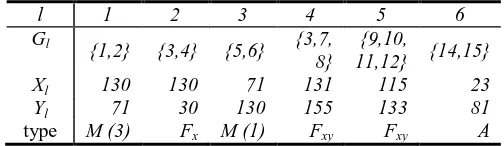
Let us now apply algorithm Approxto the instance of the 2-component vector scheduling problem constructed from the problem instance given in our example. Initially all the five processors are type A. The first two iterations tasks 1 and 2 are assigned to processor 1and the processor becomes type Fx. The next two iterations tasks 3 and 4 are assigned to processor 2and the processor becomes type Fx. The next 8 iterations assign tasks to each of the remaining processors and all the processors become type Fx or Fy. The status of all the processors after the first 12 iterations is given in Table 3.
Table 3: Assignment of the First Twelve Tasks in our Example.
l 1 2 3 4 5 6
G_l {1,2} {3,4} {5,6} {7,8} {9,10} {11,12}
X_l 130 131 71 70 105 10
Y_L 71 50 130 130 28 105
Type Fx Fx Fy Fy Fx Fy
When the algorithm considers task 13, none of the processors are type A. So the algorithm selects a processor typeFx and one type Fy. Let’s say the algorithm sets j=1 and k=3. Processors j and k are incompatible as Xj+Xk=130+71>200=2L and Yj+Yk=71+130>200=2L. So the algorithm matches these processors to each other (see Table 4) and then selects two unmatched processors (one type Fx and the other type Fy). Lets say the algorithm sets j=2 and k=4. This pair is y-compatible. The algorithm transfers task 3 from processor j to k and processor j becomes type A. Task 13 is then assigned to processor j. As a result of this processor j remains type Fx and processor k becomes type Fxy (see Table 4).
When the algorithm considers task 14, none of the processors are type A so the algorithm selects a processor type Fx and one type Fy. Let’s say the algorithm sets j=5 and k=6. This pair is xy-compatible. The algorithm transfers tasks 11 and 12 from processor k to j. Processors j becomes type Fxy and processor k becomes type A. Then task 14 is assigned to processor 6 and processor 6 remains type A. In the next iteration task 15 is assigned to processor 6 (which is type A) and the processor remains type A. Table 4 shows the final assignment of the tasks to the processors.
Lemma 1:Algorithm Approx generates a schedule with finish time at most 2Lfor any 2-component vector scheduling problem instance, in O(n+m) time.
Proof: First we establish correctness and prove the approximation bound. Then we prove the time complexity bound. If at each iteration a jobs is assigned to a processor type A, then at the end of the algorithm every processor will be of type A, Fx, Fy orFxy, and the schedule will have makespan at most 2L. The proof is by contradiction. Suppose that there are problem instances for which the above algorithm fails to assign a job to a processor. Let I be any of these instances. As our algorithm processes instance I it will eventually encounter a job i that cannot be assigned to any of the processors. Consider now the first time during the ith iteration when the condition of the
while statement was true, i.e., none of the processors were type A. Let r be the number of processors that are type Fxy or matched.
Table 4: Final assignment of all the tasks in our example.
l 1 2 3 4 5 6
Gl {1,2} {3,4} {5,6} {3,7, 8}
{9,10,
11,12} {14,15}
Xl 130 130 71 131 115 23
Yl 71 30 130 155 133 81
type M (3) Fx M (1) Fxy Fxy A
We claim that r is less than, the number of processors, m, and that there must be at least one unmatched type Fx processor and one unmatched type Fy processor. The proof of the claim follows from the fact that if there were zero type A processors and zero type Fx processors, then the sum of the y-component of all of the jobs previously assigned to the processors would exceed mL, which contradicts the definition of L. Similar arguments can be used to prove that there must be at least one processor type A and one processor type Fy.
So, there is at least one processor j type Fx and one processor k type Fy. There are several cases depending on the compatibility of processors j andk.
Case 1: Processor j and k are incompatible.
In this case processors j and k will be matched to each other and the value of r increases by two. By using arguments similar to the ones above one can show that the new value for r is less than m and there is an unmatched processor j type Fx and another unmatched processor k type Fy. There are no type A processors and the condition of the while Statement must hold at the next iteration.
Case 2: Processor j and k are xy-compatible.
Case 3: Processors j and k are x-compatible.
Since processor j is type Fxwe know that L <Xj≤ 2L and 0 ≤ Yj≤ L, and since processor k is type F_y we know that 0 < Xk≤ L and L ≤ Yk≤ 2L. Since processors j and k are x-compatible and all jobs have their y-component smaller than L, we know that we can reassign at least one job from processor k to processor j. The algorithm reassigns a subset of jobs assigned to processor k to processor j. When no more jobs can be reassigned from processor k to processor j, we know that processor j is type Fxy, because processors j and k are x-compatible, processor j is type Fx, and processors j and k were not y-compatible to begin with. Processor k will either become type A or remain type Fy, and r will be increased by 1. In the former case task i is assigned to processor k. But this contradicts the previous assumption that task i could not be assigned. In the latter case by using arguments similar to the ones above one can show that the new value for r is less than m and there is an unmatched processor j type Fx and another unmatched processor k type Fy. There are no type A processors and the condition of the while statement holds at the next iteration.
Case 4: Processors j and k are y-compatible.
The proof for this case is omitted as it is similar to the one for Case 3.
In the above four cases either we contradict our earlier assumption or the value of r increases by at least one and the condition of the while loop will hold. After no more than m iterations (of the while loop) we either reach a contradiction or r becomes larger than m. But as we stated before, this leads to a contradiction.
This completes the proof of correctness and the approximation bound. To complete the proof of the lemma, we need to prove the time complexity bound.
An implementation detail we have not discussed is that we keep four (doubly-linked) lists of processors, one for each type of processors, and an array (indexed by a processor number) pointing to the elements in the doubly-linked list. We also keep the number of processors of each type. Therefore, finding a processor of certain type, know if there are zero processors of certain type, or deleting/adding a processor of a certain type, can be easily implemented to take constant time. Every time we iterate through the while loop we will increase, r, the number of matched processors plus the number of type Fxy processors by at least one. In the proof of the first part of this lemma we show that r will always be smaller than r-1. Since r is never decreased, it follows that the while loop is executed at most r-1times. The body of the while loop can be easily implemented to take constant time. The for-statement is executed n times and each time it takes constant time, excluding the time taken by the while loop which is being counted separately. Therefore the time complexity is O(n+m). This concludes the proof of the lemma.
There are problem instances for which our algorithm, or for that matter any algorithm, does not generate solutions with makespan significantly smaller than 2L. For some of those problem instances the optimal makespan is close to 2L. Therefore, there may exist simple algorithms to construct schedules with makespan significantly better than 2*OPT, where OPT is the optimal makespan. As we shall see, even if such algorithms exist they will have minimal impact in our analysis.
3.APPROXIMATING THE BIPARTITE PROBLEM.
Let us outline our four-phase approximation algorithm.Our approach begins by assigning tasks to the processor where they are to be processed in such a way that the computing and communication time are balanced (suboptimally), and then the actual schedules are constructed. The schedules generated by our algorithm consist of two parts: a communication schedule that specifies when all the communications take place, and a computation schedule that specifies when all the processing of the tasks takes place. We say that we are approximating the problem by ``restriction'' as our initial approach performs first all the communications and then, at a separate time, all the computation. But, since the tasks will be processed in the same order in which their data arrives at the in-channel associated with the processor, then it may be possible to overlap at least portions of these schedules. So our approximation technique is actually ``restriction'' followed by a posteriori ``overlapping''. Our general approach is as follows.
Determine the processor where each task i is to be executed andidentify the corresponding in-channel to be used to receive the data for task i.
Determine the out-channel to be used to send the data for task i.
Construct the communication schedule Comm, i.e., determine the actual time when the data required by the tasks is to be sent from the storage nodes via the out-channel to the receiving processing nodes via the in-channel.
Construct the computation schedule Comp, i.e., determine the actual time when each task is to be processed.
Step 1: Determine the processor and in-channel to be used to process and receive the data for each task. This is accomplished by constructing a schedule S1 (by the algorithm given in Section 2.3.1) for the 2-component vector scheduling problem P1 defined below. Let p be the total number of processors (as well as the number of in-channels) at the processing nodes, i.e., p =Σj=w+1,…, mnj. The first nw+1 processors are located at node w+1, the next nw+2 processors at node w+2, and so on.
We construct the instance P1 of the 2-component vector scheduling problem as follows. For each task i we define job i with Ti as its x-component and di as its y-component. Define
T= min {Σ ti/ p, max {ti} }, D = min {Σdi / p}, max{di} }, and L = max {T, D }.
Clearly the x-component and y-component of each one of the tasks is a value between 0 and L. The sum of the x-component and y-x-component of all the tasks is at most pL, respectively. We construct a schedule S1 for the instance P1 by using the linear time algorithm given in Section 2.3.1. All the tasks assigned to the same machine in schedule S1 are assigned to the same processor for their execution and their data is to be received by the in-channel corresponding to the processor.
As we established in Section 2.3.1 all the tasks assigned to the same machine in schedule S1are such that the sum of their x-component is at most 2L and the sum of their y-component is at most 2L. Therefore, every processor will be running tasks for at most 2L time units, and every in-channel will be receiving data for at most 2L units of time (later on we construct the actual schedules specifying when these operations will take place).
Name the four processors at node 4 as processors 1, 2, 3, and 4; and the two processors at node 5 as processors 5 and 6. The corresponding in-channels are referred to as I1, I2, I3, I4, I5, and I6. In Section 2.3.1 we applied our 2-component vector scheduling algorithm to the instance given in our example. This is instance P1 defined above and the resulting schedule is S1. The tasks assigned to the six processors (represented by the sets Gj) are given in Table 5 (constructed from Table 4). We use Tj (Dj) as the sum of the processing (communication) time requirements of the tasks assigned to processor j.
Table 5:Task Assignments to Processors (and corresponding In-channels) for Schedule S1 for our
Example.
j I1 I2 I3 I4 I5 I6
Gj {1,2} {4,13} {5,6} {3,7, 8}
{9,10,
11,1} {14,15}
Tj 130 130 71 131 115 23
Dj 71 30 130 155 133 81
Step 2: Now let’s determine the out-channel to be used to send the data for each task to the processor where the task
is to be executed. Let q be the total number of out-channels in the storage nodes, q = Σj=1, …, wcj (remember cj is the number of out-channels in node j). For every storage node k, our algorithm partitions the tasks' data files stored in it into cj groups. The data for each task assigned to each group is to be sent via a different out-channel. The partitioning should be such that the sum of the communication times of all the data for the tasks assigned to the out-channels is balanced as much as possible. It is well known that this partitioning problem is NP-hard under the assumption that all the data needed by a task has to be transmitted using the same channel4. For this version of the problem, one can generate a near-optimal solution by modeling the partitioning problem as an instance of the problem of scheduling independent jobs on identical machines (which is the same as the single-component vector scheduling problem). Each task corresponds to a job and the execution time of each job is the time required to transmit the data for the corresponding task. We can use any of the scheduling algorithms discussed in the Section 2.1 to generate a near-optimal schedule which is then used to obtain near-optimal balanced partitions. If we use list scheduling [9] then one can construct schedules with makespan at most 2 times the makespan of an optimal schedule in O(n log m) time. On the other hand, LPT generates schedules with makespan (finish time) at most 4/3 - 1/(3m) times the makespan of an optimal schedule [10]in O(n log n) time. We use P2 to denote the collection of scheduling problems just defined and S2 to denote the set of schedules generated.
For our example, the out-channel at node 1is namedO1, the three out-channels at node 2 as O2, O3, and O4, and the two of node 3 as O5 and O6. Using the task indices as the list (for the list scheduling algorithm) one can easily construct list schedules for each of the three storage nodes when considering the di values as the processing times for the jobs. Table 6 shows a possible list schedule (assignment of tasks to the out-channels) at each node. Note that one may generate many different list schedules. Our results hold, no matter which list schedule is generated. The total communication time of the tasks is shown in the next column.
Table6: Assignment of Tasks to Out-channels for our Example.
Node
Out-channel
Tasks Assigned
Total Comm.
Time
1 O1 {1,2} 71
2 O2 {3,6} 95
2 O3 {4,7,9} 155
3 O4 {5,9,10} 88
3
O5
{11,13,
14,15} 131
3 O6 {12} 60
4
To summarize the first two steps, we have determined for every task i the out-channel to be used to send the data it needs as well as the in-channel to receive it, and the corresponding processor to execute the task. We just need to determine the actual time when the data for each task is to be transmitted and the time at which the tasks are to be processed in such a way that there are no communication conflicts, i.e., the data for two or more tasks is not being sent or received by the same channel at the same time, and the processing of a task cannot start before the processor has all the task's data. In other words, we need to construct the communication schedule Comm and the computation schedule Comp.
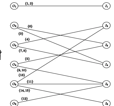
Step 3:The timing of all the communication events is obtained by modeling the problem as an instance of the openshop scheduling problem. Before defining the openshop instance P3 it is convenient to begin by defining the bipartite graph G consisting of the set of vertices S and P. Each vertex in set S represents a storage node and one of its communication out-channels. Similarly, each vertex in set P represents a processor in a processing node and its corresponding communication in-channel. At this point our algorithm knows the out-channel (Step 1) and in-channel (Step 2) for the transmission of the data for each task i. This information is used to define the set of edges in the graph (for our example see Fig. 2). There is an edge from a vertex i in S to a vertex in j in P if there is at least one task using the out-channel i and the in-channel j. Note that several tasks may be represented by the same edge. So we label each edge by the set of tasks it represents (Fig. 2). The weight of the edge is the total communication time needed to transmit the data for all the tasks represented by the edge. Each node in S represents a job and each node in P represents a machine in the instance of the openshop problem P3 we construct. We define as pi,j the weight of the edge joining vertex i in S to vertex j in P, and zero if such edge does not exist. Let xi be the sum of the weight of the edges incident to vertex i in S, i.e. Σjpi,j, let yj to be the sum of weight of the edges incident to vertex j in P, i.e. Σipi,j. We define t as max{xi, yj }. From Ref. [13]we know that there is a preemptive communication schedule S3 with makespan t for P3 and schedule S3 can be constructed in polynomial time5. From schedule S3 one can easily construct schedule Comm that gives the specific times when the data for task i must be transmitted from the storage node where it resides to the processing node where it is to be processed using the channels that have been previously selected.
For our working example, Table 7 shows the execution time requirements for the jobs (pi,j) computed from the bipartite graph given in Fig. 2 and and the tasks' communication times given in Table 2. This is problem instance P3. A possible schedule S3 constructed by the algorithm given in Ref.[13] for instance P3 defined in
5
Note that this claim has been independently established is many papers. We use Ref. [13] because their algorithm to generate such schedules is asymptotically faster than all known algorithm for this problem.
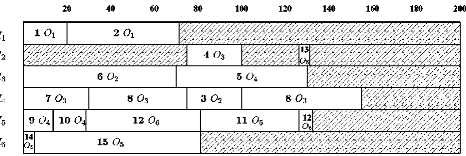
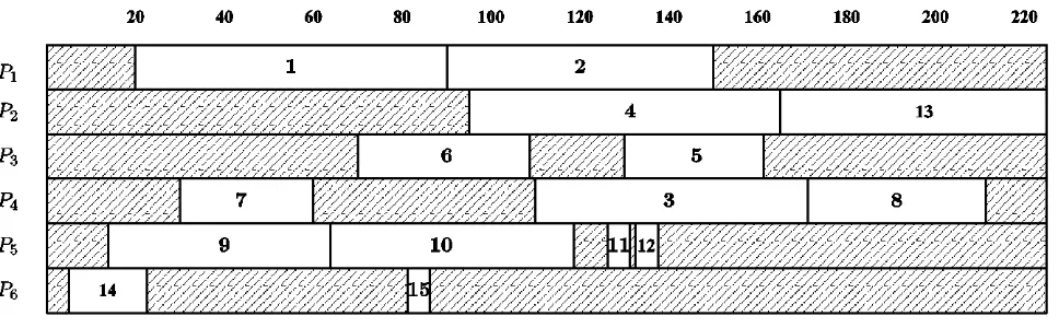
Table 7 is given in Fig. 3. The horizontal axis represents time and the rows correspond to the in-channels (or the corresponding processors). Each block assignment is labeled with a task index and the out-channel used in the communication. Note that the schedule is preemptive, so a task index may be assigned to two or more time intervals (block assignments). However, at no point in time an out-channel is used by two or more tasks, simply because the out-channel can only be sending one data set at a time. In Appendix I we give the schedule with respect to the out-channels. I.e., the horizontal axis represents time and the rows correspond to the out-channels. Each block assignment is labeled with a task index and the in-channels used in the communication.
Figure 2: Bipartite Graph Constructed for our Example.
Table 7: Openshop Instance P3 for our Example.
Jobs\Machines 1 2 3 4 5 6 Xi
1 71 - - - - - 71
2 - - 70 25 - - 95
3 - 25 - 130 - - 155
4 - - 60 - 28 - 88
5 - 5 - - 45 81 131
6 - - - - 60 - 60
Yj 71 30 130 155 133 81
Figure 3: In-channel Communication Schedule Constructed for problem P3 for our Example.
processor j before task i have completed processing and t2 is the time at which all the data for task i is available at processor j.
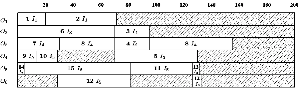
Using the communication schedule given in Fig. 3 one constructs (as defined above) the computation schedule for our example. The resulting schedule is given in Fig. 4.
Our four-phase algorithm is formally defined below:
Four-Phase Algorithm
Let q = Σj=1,…,cnj; //number of out-channels
Let p = Σj=c+1,…,mnj; //number of processors and in-channels Step 1: Determine the processor where each task i is to be
executed and identify the corresponding in-channel to be used to receive the data for task i.
Construct the instance P1 of the 2-component vector scheduling problem as follows.
For each task i we define its x-component asti and its y-component as di.
Let T=min { Σti / p }, max {ti} }, Let D =min { Σdi/ p, max {di} } Let L =max { T, D }
Construct a schedule S1 for P1 via the algorithmgiven in Section 2.3.1;
Assign all the tasks corresponding to the jobs scheduled on the same machine in S1 to the same processorand corresponding in-channel.
Step 2: Determine the out-channel to be used to send the data for task i.
For each storage node k define an instance of the problem of scheduling independent jobs on
identical machines. For each task stored at node k, define ajob with execution time equal to dj, the timerequired to transmit the data fortask j, and definethe number of machines as ck.
Use list scheduling[9]to construct a non-preemptive schedule for each storage node.
The combined problems are called P2 and the set of schedules generated is S2.
All the tasks corresponding to the jobs assigned to the same machine in S2 will be using the same
out-channel.
// At this point we know for every task i the // out-channel and in-channel used to transmit the // data it needs, as well as the processor that will // execute the task.
// In the next steps we determine exactly when all of // these operations take place.
Step 3: Construct the communication schedule Comm, i.e., determine the actual time when the datarequired by the tasks is to be sent from the storagenode via the out-channel to the receiving processing node via the corresponding in-channel.
Define the bipartite multigraph G=(S P,E).
There is a vertex in S for each storage node and one of its communication out-channels.
There is a vertex in P for each processor in a processing node and its correspondingcommunication
in-channel.
There is an edge from vertex i in S to vertex in j inP if there is at least one task using both the out-channel i and the in-channel j.
Label each edge by the set of tasks it represents. The weight of the edge { i, j } denoted by pi,j isthe total communication time needed to transmit the data for the tasks represented by the edge.
Let xi = Σjpi,j andyi = Σipi,j. Let t= max { xi,yj }.
Construct the preemptive schedule S3 for P3 with makespan t(algorithm in Ref. [13]).
Figure 4: Computation Schedule Constructed for our Example.
Step 4: Construct the computation schedule Comp. Construct the schedule Comp that specifies for each
processor the order in which the tasks assigned to it are to be processed. The ordering foreach processor is the same one as the order in which their data arrivesto the processor via the in-channel.
End of Four-Phase Algorithm
Theorem 1:The time complexity for the four-phase
algorithm is O(np (p+log q)) and the algorithm generates schedules with makespan at most four times themakespan of an optimal schedule.
Proof:The number of tasks, processors (in-channels) and out-channels isn, p, and q, respectively.In Step 1 we construct aninstance of the 2-component scheduling problem.Constructing this instance takes O(n+ p) time andconstructing a schedule for the instance takesO(n+ p) time (Section 2.3.1).
Step 2 constructs q instances of the identical machine scheduling problem. This can be accomplished in O(n+q) time and constructing list schedules for all instances takes O(n log n) time [10].
Assigning the actual time when the data for each task is to be transmitted from the out-channel to the in-channel is determined by solving an instance of the openshop preemptive scheduling problem. Constructing the instance P3 of the openshop problem takes O(n+p+q) time. Constructing the schedule S3 for the openshop instance takes O(np (p+log q)) time, as the number of processors is p, the number of jobs is q and the number of non-zero tasks is n)[13].
Step 4 takes time O(n+q), as one uses the ordering of the data arriving to each processor.
Hence, the overall time complexity is dominated by the solution to the instance P3 of the openshop problem, which takes O(np (p+log q)) time.
Let us now determine the approximation ratio for our algorithm. The total time required to process the tasks (makespan of the computation schedule Comp) is at most 2L, where L is a lower bound for the total time required for the processing of the tasks by the p processors and a lower bound for the total time required to receive all the data by the p in-channels. The total time required to send all the data for the tasks by the q processors is at most 2 L', where L' is a lower bound for the time required to send all the data by the q out-channels. The solution to the openshop problem is a communication schedule, Comm, with makespan at most max { 2L, 2L' }. Since an optimal makespan for the whole problem, f*, is at least max {L, L'}, it then follows that our two schedules (Comm and Comp) have makespan at most 4 f*. This concludes the proof of the theorem.
Note that we could have used different approximation algorithms in Steps 2 and 3 that would result in a different overall approximation ratio. Suppose that in Step 1 and 2 we use approximation algorithms that generate schedules with makespan f1≤ k1f1* and f2≤ k2f2*, respectively. Then the approximation ratio for the overall algorithm would be k2+ max { k1, k2}.
suppose that we use an approximation algorithm for the openshop problem that generates solutions such thatf3≤k3f3*. Then the approximation ratio for the overall algorithm becomes k2 + k3max { k1,k2 }, wherek1 and k2 are as define above. Table captions appear centered above the table in upper and lower case letters. When referring to a table in the text, no abbreviation is used and "Table" is capitalized.
4.GENERALIZATIONS
In this section we consider several generalizations of our problem. The first one addresses the problem when the tasks required data resides in more than one node, the second one deals with the problem when tasks have output files to be stored at the storage nodes, and the third one addresses the case when the output files for each task may reside in multiple nodes. In all cases we show how to extend our approximation algorithm to provide constant ratio approximations to these problems.
4.1. Multiple Data Files
Consider now the situation when data for each task resides in one or more storage nodes. We use the vector Si to indicate the nodes where the task's data resides. Corresponding to each vector Si there is a vector Di whose jth component indicates the time required to transfer the data for task Si stored at the node specified by the jthcomponent of the Si vector.
The approximation algorithm for the basic case given in the Section 3 can be easily generalized to solve this problem. The first phase is exactly as before, except that di is equal to the sum of all of the values in vector Di. Remember that in this phase we determine the processor where each task is to be processed so that the communication and processing times are balanced. The second phase, where we determine the out-channel for the data for each program, is in principle identical to the one in Section 3. The difference is that each task uses an out-channel on each node where its data resides. The third step is identical to the one in Section 3, since we know for each data file its out-channel and in-channel. The fourth phase, where we determine the processing order for the tasks, is identical to the previous one, except that we have to take into consideration that all the data for a task must arrive at the processing node before one can begin the processing of the task.
The approximation ratio for this case is identical to the one in the Section 3. The time complexity bound is similar to the previous one after taking into consideration the fact that there is more input in this case than for the basic problem.
4.2. Tasks Generating Output Files.
Let’s consider the case where each task i creates an output file which is to be stored at a given storage node si’. The restriction is that the file will be available for transmission only after the processing of the task has completed. Letoi
the time required to transfer the file. This problem is significantly harder than the basic one as one must not only balance the transfer time (for the input data) and the processing time, but also the transfer time for the output files.
The idea behind the approximation algorithm is similar to the one for the basic case. One important difference is that instead of using an approximation algorithm for the 2-component vector scheduling problem we use one for the three-component problem.
The schedules generated by our algorithm consist of three parts: an input communication schedule for the input data communications, a computation schedule for the processing of the tasks, and anoutputcommunication schedule for transferring the output files. We initially classify our approximation technique as ``restriction,'' since we construct three separate schedules. Then we try to overlap the three schedules as much as possible. Since the tasks are processed in the same order in which their data arrives in the in-channel associated with the processor, most of the time it is possible to overlap at least portions of the first two schedules. However the transmission of the output files might not be in the same order in which the processing of the tasks is performed, so the overlapping of the computation and the output communication schedule is limited and in the worst case non-existent. So our approximation technique is ``restriction'' followed by a posteriori ``overlapping''. The general approach for our algorithm is as follows.
Determine the processor where each task i is to be executed, identify the corresponding in-channel to be used to receive the input data for task i, and identify the out-channel to set the output file for task i.
Determine the out-channel to be used to send the input data for all tasks.
Construct the input communication schedule In-Comm, i.e., determine the actual time when the input data required by the tasks is to be sent from the storage node via the out-channel to the receiving processing node via the in-channels. Construct the computation schedule Comp, i.e., determine the actual time when each task is to be processed.
Determine the in-channel to be used to receive the output file for task i.
Construct the output communication schedule Out-Comm, i.e., determine the actual time when the output file generated by the tasks is to be sent from the processing node via the out-channel to the receiving storage node via the in-channels.
problem; and the forth one, the simplest one, as the processing ordering for the tasks is determined by the ordering of the data arriving to the processor. Step 5 is implemented by scheduling sets of independent jobs on sets of identical machines; Step 6 is implemented by solving an openshop scheduling problem. In what follows we explain all the steps in our procedure.
Step 1:Determine the processor, in-channel, and out-channelto be used to process,receive the input data, and send the output file for each task, respectively.This is accomplished by constructinga schedule S1 by any approximation algorithmfor the three-component vector scheduling problem P1 defined below.Let p be the total number of processors (as well as the number ofin-channels and out-channels)at the processing nodes, i.e.,
p = Σj=w+1, …, m n_j.
The first nw+1 processors are located atnode w+1, the next nw+2 processors at node w+2,and so on.
We construct the instance P1 of the three-component vector scheduling problem as follows.For each task i, we define job i with its x-component as ti,its y-component as di, and its z-component as oi.Define
T= min { Σti / p, max {ti } }, D= min { Σdi /p, max {di } }, O = min { Σoi /p, max { oi } }, and L = max { T, D, O }.
Clearly the x-component, y-component and z-componentof each one of the tasks is a value between 0 and L. The sumof the x-component, y-component, and z-component of all the tasksis at most pL,respectively.We construct a schedule S1 for the instance P1by using any polynomial time approximation algorithm for the three-componentvector scheduling problem.All the tasks assigned to the same machine in schedule S1are assigned to the same processor for their executionand their data is to be received by thein-channel corresponding to the processorand the output file is to be sent using the out-channel correspondingto the processor.
There is an approximation algorithm that assigns tasks to the same machine (in schedule S1) in such a way that thesum of their x-component is at most 3L,sum of their y-component is at most 3L and thesum of their z-y-component is at most 3L (Section 2.3).Therefore,every processor will be running tasks for at most 3Ltime units, every in-channel will be receiving data forat most 3L units of time, and every out-channel willbe sending output data for at most 3L units of time(later on we specify the actual schedules when theseoperations take place).
Step 2:Now let’s decide the out-channel to be used to send the data for each taskto the processor where the task is to be executed.Let q be the total number ofout-channels in the storage nodes,q = Σj=1, …, wcj (remembercj is the number of out-channels in node j).For every storage node k, our algorithmpartitions the tasks' data stored in itinto cj groups.The data for each task assigned to each group is to
be sentvia a different out-channel to the nodewhere the processing of the task will take place.This partitioning should be in such a way that the sum of the communicationtimes of all the data for the tasksassigned to the out-channels is balanced as much as possible, as this willdecrease the total communication time.We use the same algorithm as in the Section 3 forthis step.
To summarize the first two steps, we have determined for every task i the out-channel to be used to send the input data it needs as well as the in-channel that will receive it, and the corresponding processor where the task will be executed. We need to determine the actual time when the data for each task is to be transmitted and the time at which the tasks are to be processed in such a way that there are no communication conflicts, i.e., the data for two or more tasks is not being sent or received by the same channel at the same time, and the processing of a task cannot start before the processor has all the task's data. In other words, we need to construct the input communication schedule, In-Comm, and the computation schedule Comp, and the output communication schedule Out-Comm.
Step 3:The timing of all the communication eventsin the In-Commschedule is obtained by modeling theproblem as an openshop scheduling problem and then constructing a schedule for itas we did in Section 3.
Step 4:The computation schedule Comp is constructed as in Section3.
Now we know the out-channel and the in-channel for all the output data files. The actual timing for all the communications (Out-Comm schedule) is determined in the next steps.
Step 5:In this step we determine the in-channel for each output file. This operation isexactly like Step 2 in Section 3, except that we use the in-channels in the storagenodes and the tasks' output files.
Step 6:In this portion we construct the Out-Comm schedule. This is exactly asStep 3 in Section 3, but with the out-channels located at the processing nodesand the in-out-channels located at the storage nodes.
The above steps can be easily formalize into the six-phase
approximation algorithm. The following theorem can be established by using arguments similar to those in used in the proof of Theorem 1.
Theorem 2:The time complexity of algorithmsix-phase is O(np (p+log q) + nq (q + log p)) and the algorithm generates schedules with makespan at most six times the makespan of an optimal schedule.
ratio k3. Suppose that in Step 5 we use an approximation algorithm that generates schedules with makespan
f5≤ k5f5 *
. Then the approximation ratio for the algorithm is k2 + k3 * max { k1 ,k2 }+ k3 *max { k1 , k5 }.
V.3. Multiple Output Files
Suppose now that each task creates multiple files to be stored in one or more storage nodes. In this case we use the vector Si’ to indicate the nodes where the task output files will be stored. Corresponding to each vector Si’ there is a vector Di’ whose jthcomponent indicates the time required to transfer the data for task i stored at the node specified by the jth component of vector Si’.
We extend the approximation algorithm given in Section 4.2 to this problem as follows. The main differences are in the last two steps which are now similar to the ones for multiple input files for the algorithm given in Section 4.1.
The approximation ratio for this case is identical to the one in the Section 4.2. The time complexity bound is similar to the one in Section 4.2 after taking into consideration the fact that the size of the input is larger than for that problem.
5.DISCUSSION
We have presented a four-phase algorithm that takes O(np (p+log q)) time and generates schedules with makespan at most four times the makespan of an optimal schedule for the case when the set of nodes is partitioned into storage and processing nodes. Recall that n is the number of tasks, p is the number of channels in the storage nodes, and q is the number of channels in the processing nodes. We have shown that the time complexity bound can be decreased to O(n log q), but then we can only guarantee solutions that are within six times the optimal one. We also showed how to generalize our algorithm for the case when there are output files for each task as well as for the case when there are multiple input data files and output data files for each task.
Another interesting problem is to transform our algorithms to distributed ones. The portion that is transformable to a distributed on-line algorithm is the solution to the openshop problem by using the algorithm developed by Anderson and Miller [20]at the expense of generating solutions farther from optimal. However one needs to solve on-line the other scheduling problems. List scheduling is an on-line algorithm, but it is not a distributed one. Transforming it to a distributed one as well as transforming our algorithm for the 2-component vector scheduling problem, while maintaining the same approximation ratios and at the same time decreasing significantly their time complexity bounds are challenging open problems.
Another interesting variation of our problem is when nodes may be used for storage and processing, as well as
when the communication times depend on the source and destination nodes and the processing speeds of the processors depends on the task being processed. These are more realistic variations of our problem; however, it is not clear whether or not there exist efficient constant ratio approximation algorithms for these problems.
A conclusion section must be included and should indicate clearly the advantages, limitations, and possible applications of the paper. Although a conclusion may review the main points of the paper, do not replicate the abstract as the conclusion. A conclusion might elaborate on the importance of the work or suggest applications and extensions.
REFERENCES
[1] K. Ranganathan and I. Foster, "Computation and Data Scheduling in Distributed Data Intensive Applications," in Proc. 11th IEEE Symposium on High Performance Distributed Computing (HPDC 02), July 2002.
[2] O. Beaumont, A. Legrand and Y. Robert, "Optimal Algorithms for Scheduling Divisible Workloads on Heterogeneous Systems," in Proc. 17 International Parallel and Distributed Processing Symp, (IPDPS 2003), 2003.
[3] P. Lampsas, T. Loukopoulos, F. Dimopoulos and M. Athanasiou, "Scheduling Independent Task Scheduling in Heterogeneous Environments under Communication Constraints," in Proceedings of the 7th International Conference on Parallel and Distributed Computing, Applications and Technologies (PDCAT 2006), 2006.
[4] T. Loukopoulos, P. Lampsas and P. Sigalas, "Improved Genetic Algorithms and List Scheduling Techniques for Independent Task Scheduling in Distributed Systems," in Proceeding of the 8th International Conference on Parallel and Distributed Computing, Applications and Technologies (PDCAT 2007), 2007.
[5] H. Casanova, A. Legrand, D. Zagorodnov and F. Berman, "Heuristics for Scheduling Parameter Sweep Applications in Grid Environments," in Heterogeneous Computing Workshop, 2000.
[6] K. Kaya, B. Ucar and C. Aykanant, "Heuristics for Scheduling File-Sahring Tasks on Heterogeneous Systems With Distributed Repositories," Journal of Parallel and Distributed Computing, vol. 67, pp. 271 - 285, 2007.
[7] N. Nobrega, L. Assis and F. Brasileiro, "Scheduling CPU-Intensive Grid Applications Using Partial Information," 2008.
[8] F. A. B. da Silva and H. Senger, "Improving Scalability of Bag-of-Tasks Applications Running on Master-Slave Plataforms," Journal of Parallel Computing, vol. 35, no. 2, 2009.
1563-1581, 1966.
[10] R. Graham, "Bounds on Multiprocessing Timing Anomalies," SIAM Journal of Applied Math., vol. 17, no. 2, pp. 416-429, 1969.
[11] J. Y.-T. Leung, Handbook of Scheduling: Algorithms, Models, and Performance Analysis, Chapman & Hall/CRC, 2004.
[12] T. F. Gonzalez, Handbook of Approximation Algorithms and Metaheuristics, Chapman & Hall/CRC, 2007.
[13] T. Gonzalez and S. Sahni, "Open Shop Scheduling to Minimize Finish Time," Journal of the ACM, vol. 23, no. 4, pp. 665 - 679, 1976.
[14] D. B. Shmoys, C. Stein and J. Wein, "Improved Approximation Algorithms for Shop Scheduling Problems," SIAM J. Comput., vol. 23, pp. 617 - 632, 1994.
[15] C. Chekuri and S. Khanna, "On Multidimensional Packing Problems," SIAM Journal on Computing, vol. 31, no. 1, pp. 35-41, 2004.
[16] H. Kellerer and V. Kotov, "An Approximation Algorithm with Absolute Worst-case Performance Ratio 2 for Two-dimensional Vector Packing," Operations Research Letters, vol. 31, no. 1, pp. 35-41, 2003. [17] R. Anderson and G. Miller, "Optical Communications
for Pointer Based Algorithms," TRCS, CRI 88-14, USC, 1988.
[18] R. Cole and J. Hopcroft, "On Edge Coloring Bipartite Graphs," SIAM J. on Computing, vol. 11, no. 3, pp. 540-546, 1982.
[19] H. Gabow and O. Kariv, "Algorithms for Edge Coloring Bipartite Graphs and Multigraphs," SIAM J. Computing, vol. 11, pp. 117-129, 1982.
[20] R. Cole, K. Ost and S. Schirra, "Edge-Coloring Bipartite Multigraphs in O(E log D)," Combinatorica, vol. 21, pp. 5-12, 2001.
Appendix I
In Fig. 3 you will find the schedule S3 constructed for the algorithm given in Ref. [13] for the instance P3 of the openshop problem given in Table 7. Fig. 5 you will find the same schedule, but with respect to the out-channels. I.e., the horizontal axis represents time and the rows correspond to the out-channels. Each block assignment is labeled with a task index and the in-channel used to receive the data communication.
Biography
Professor Gonzalez was born in Monterrey, Mexico. He received a BS degree in computer science from the ITESM (1972). He received his Ph.D. degree from the University of Minnesota (1975). He has been member of the faculty at OU, Penn State, and UT Dallas, and has spent sabbatical leave at the ITESM Monterrey (Mexico) and U. Utrecht (the Netherlands). Since 1984 he has been professor of computer science at UCSB. His main area of research activity is the design and analysis of efficient exact and approximation algorithms, deterministic scheduling, CAD, graph algorithms, computational geometry, parallel computing, and multicasting.