STRUCTURAL TIME SERIES MODEL FOR FORECASTING POTATO PRODUCTION
AN INVENTORY MODEL OF PERISHABLE PRODUCTS WITH DISPLAYED STOCK LEVEL DEPENDENTDEMAND RATE
TWO NEW BIVARIATE NEGATIVE BINOMIAL DISTRIBUTIONS AND THEIR PROPERTIES
TARDINESS OF JOBS AND SATISFACTION LEVEL OF DEMAND MAKER IN m-STAGE SCHEDULING WITH FUZZY DUE TIME
A NOTE ON ORTHOGONAL IDEMPOTENTS IN FG, G IS AN ABELIAN GROUP
TESTING OF PROPER RANDOMNESS OF THE NUMBERS GENERATED BYKENDALL AND B. BABINGTON SMITH: t-TEST
ONTHE DIOPHANTINE EQUATION x = b x+k
STATISTICAL ASSESSMENT OF ADOPTION OF SELECTED AGRICULTURALTECHNOLOGIES IN CHHATTISGARH STATE
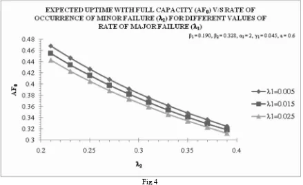
AVAILABILITY MODELING AND BEHAVIORAL ANALYSIS OF A SINGLE UNIT SYSTEM UNDER PREVENTIVE MAINTENANCE AND DEGRADATION AFTER COMPLETE FAILURE USING RPGT
THERMAL INSTABILITY IN ANISOTROPIC POROUS MEDIUM LAYER SATURATED BYANANO-FLUID : BRINKMAN MODEL
CERTAIN CLASSES OF MESOMORPHIC FUNCTIONS WITH RESPECTTO ( ) SYMMETRIC POINTS
THE STUDY OF SERIAL CHANNELS CONNECTED TO NON-SERIAL CHANNELS WITH FEEDBACK AND BALKING IN NON-SERIAL CHANNELS AND RENEGING IN BOTHTYPES OF CHANNELS D.P. Singh and Deo Shankar
Deep Shikha, Hari Kishan and Megha Rani
Swagata Kotoky, Subrata Chakraborty
Meenu Mittal, T.P. Singh, Deepak Gupta
Sheetal Chawla, Jagbir Singh
Brajendra Kanta Sarmah, Dhritikesh Chakrabarty
Hari Kishan and Sarita
Roshan Kumar Bharadwaj, S.S. Gautam and R.R. Saxena
Sarla, Vijay Goyal
Ruchi Goel, Sudhir Kumar Yadav and Naresh Kumar Dua
A. Senguttuvan and K.R. Karthikeyan
Satyabir Singh, Man Singh and Gulshan Taneja a P i S i
j, k EXISTENCE OF SOLUTIONS OF STOCHASTIC NEUTRAL
FUNCTIONAL DIFFERENTIAL EQUATIONS WITH STATE DEPENDENTDELAY
DEVELOPMENT OF INVENTORY MODEL OF DETERIORATING ITEMS WITH LIFE TIME UNDER TRADE CREDIT AND TIME DISCOUNTING
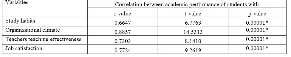
CASUAL MODEL OF ACADEMIC PERFORMANCE OF STUDENTS OF SECONDARY SCHOOLS-A STRUCTURAL EQUATION MODELING APPROACH
B-MODEL AND FM-MODEL IN STOCHASTIC PROCESSES
REVIEW ON WORD SENSE DISAMBIGUATION TECHNIQUES
ON NEW WEIGHTED DIFFERENCE-DIVERGENCE MEASURES THEIR INEQUALITIES, CONCAVITY AND NON-SYMMETRY
STOCHASTIC MODEL TO ESTIMATE THE INSULIN SECRETION USING NORMALDISTRIBUTION
REVIEW ON ESTIMATION OF CORRELATION BETWEEN VARIOUS PIXELINTENSITIES OF MICROARRAYSPOTS
COST-BENEFIT ANALYSIS OF A TWO-UNIT CENTRIFUGE SYSTEM CONSIDERING REPAIR AND REPLACEMENT
AN EOQ MODEL FOR DETERIORATING ITEMS WITH RAMP TYPE DEMAND, WEIBULL DISTRIBUTED DETERIORATION AND SHORTAGES.
METHOD OF LEAST SQUARES IN REVERSE ORDER: FITTING OF LINEAR CURVE TO AVERAGE MINIMUM TEMPERATURE DATAAT GUWAHATI AND TEZPUR
WIENER LOWER SUM OF COMPLETE K – GRAPH A. Senguttuvan
Deep Shikha, Hari Kishan and Megha Rani
Dr. C. M. Math, Dr. Javali S. B.
A. Ramesh Kumar & V. Krishnan
Tanveer J. Siddiqui
Sapna Nagar, R. P. Singh
P. Senthil Kumar, K. Balasubramanian & A. Dinesh Kumar
Kalesh M Karun, Binu V. S.
Vinod Kumar and Shakeel Ahmad
Anil Kumar Sharma, Naresh Kumar Aggarwal, and Satish Kumar Khurana
Atwar Rahman, Dhritikesh Chakrabarty
Dr. A. Ramesh Kumar and R. Palani Kumar N
R
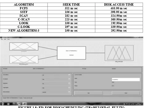
DESIGNING A FUZZY INFERENCE RULE TO OPTIMIZE OVERALL PERFORMANCE OF VARIOUS DISK SCHEDULING POLICIES
213-226
227-236
237-242
243-250
251-258
329-332
333-338
339-352
353-358
359-364
365-368
369-372
381-390 259-276
277-282
283-286
287-296
297-304
305-312
313-316
373-380
391-400
401-406
EXISTENCE OF SOLUTIONS OF STOCHASTIC
NEUTRAL FUNCTIONAL DIFFERENTIAL
EQUATIONS WITH STATE DEPENDENT DELAY
A. Senguttuvan
Department of Mathematics and Statistics, Caledonian College of Engineering, Muscat, Sultanate of Oman
ABSTRACT:
In this paper we study the existence of mild solutions for a class of stochastic neutral functional differential
equations with state dependent delay in an abstract space by using the fixed point theorem of Leray-Schauder
alternative.
Key words:Existence of solutions, Leray-Schauder fixed point theorem, Stochastic differential equations, State dependent delay.
AMS(MOS) Subject Classifications:34K40, 34A60, 34K50, 60H10, 93E03.
1. INTRODUCTION
Random differential and integral equations play an important role in characterizing many social, physical, biological and engineering problems. Neutral functional differential systems arise in many areas of applied mathematics and for this reason these systems have been extensively investigated, refer [6] in the last few decades. There are many contributions relative to this topic and we refer readers to [9, 7] and the monograph [8, 5]. Recently, much attention has been paid to existence results for partial functional differential equations with state-dependent delay, and we cite the works [17, 15, 16, 21] and similarly with unbounded delays and infinite delays we refer [18, 7, 11, 25]and monograph [4] and the references therein.The global existence results for functional integro-differential stochastic evolution equations in Hilbert space have been studied elaborately in [13]. Also Taniguchi et al. [11] established the unique solution of stochastic functional differential equations in Hilbert space using the contraction mapping principle. The existence results of differential equations have been generalized to stochastic functional differential inclusions see [10, 14, 24] using the fixed point argument.
The theory of stochastic differential equations has become an active area of research in recent years due to their numerous applications with non-deterministic nature for problems arising in mechanics, electrical engineering, medicine biology and other areas of science. In the literature, there are very few results con-cerning stochastic non-linear systems see [22, 23, 27] and references therein. The above works mainly deal with existence and controllability investigation for impulsive stochastic systems and stability of sobolev-type equations. To the best of authors’ knowledge, the problem of existence of solutions of stochastic neutral functional differential equations with state dependent delays have not been fully investigated in the literature.
Motivated by the above discussions, the results presented in the current manuscript constitute a con-tinuation and generalization of existence, uniqueness and controllability results from [10, 14, 22, 20, 11] in two ways. For one, we study the class of neutral stochastic functional differential equations with state dependent delay using an abstract phase space, together with the Leray-Schauder fixed point theorem. To the authors knowledge, this approach has not yet been applied in the study of such stochastic problems in the literature. And two, our result constitute a stochastic variant of the results concerning the existence of mild solutions in [16]; this enables one to introduce noise into the concrete models that are subsumed as special cases of the abstract system with state dependent delay being studied, thereby allowing for a more accurate description of the phenomenon.
In this paper, we are interested to study the existence of solutions of the following nonlinear neutral stochastic functional differential equation with state dependent delay in a Hilbert space,
d[x(t) +F(t, xt)] =hAx(t) +h(t, xt)idt+G(t, xρ(t,xt))dW(t), for a.et∈J := [0, a],0< a <∞,
x(t) =φ(t)∈ L0
2(Ω,B), a.e t∈J0= (−∞,0]
(1)
whereAis the infinitesimal generator of a strongly continuous semigroup of closed linear operatorS(t), t≥ 0, on a separable Hilbert spaceH with inner product (·,·) and norm k · k. x: [−r, a] →H is the initial datum such that φ(t) is the F0-measureable for allt ∈ J0, E|φ(0)|2 <∞ and R
0
−rE|φ(s)|
2ds < ∞. Let
K be another separable Hilbert space with the inner product (·,·)K and normk.kK. SupposeW(t) is a
givenK-valued Brownian motion or Wiener process with a finite trace nuclear covariance operatorQ≥0. Let L(K, H) denote the Banach space of all bounded linear operators from K into H. The histories xt
measurable mappings in H- norm andG : J×J × B → LQ(K, H), (LQ(K, H) denotes the space of all Q-Hilbert-Schmidt operators fromKintoH which is going to be defined below) is a measurable mappings in LQ(K, H)-norm. φ(t) is aB-valued random variable independent of Brownian motion W(t) with finite
second moment andρ:J× B →Ris an appropriate function.
This paper is organised as follows: In section 2, we give some basic notations and some preliminary lemmas which are more essential to this paper. In section 3, we discuss the main result. Finally, conclusion is given in section 4.
2. PRELIMINARIES
Let (Ω,F, P) be a complete probability space furnished with complete family of right continuous in-creasing sub σ-algebras {Ft, t ∈I} satisfying Ft ⊂F. An H-valued random variable is anF-measurable
functionx(t) : Ω→H,and a collection of random variables
S ={x(t, ω) : Ω→H|t∈I}
is called astochastic process. Usually, we suppress the dependence onω∈Ω and writex(t) instead ofx(t, ω) and x(t) :I →H in the place of S. Let βn(t)(n= 1,2, ...) be a sequence of real-valued one-dimensional
standard Brownian motions mutually independent over (Ω,F, P). Set
β(t) =
∞ X
n=1
p
λnβn(t)ζn, t≥0,
where λn ≥0, (n=1, 2, ...) are nonnegative real numbers and {ζn} (n=1, 2, ...) is complete orthonormal basis in K. LetQ∈L(K, K) be an operator defined byQζn =λnζn with finiteT r(Q) =P∞n=1λn <∞, ( Tr denotes the trace of the operator). Then the above K-valued stochastic processβ(t) is called a Q -Wiener process. We assume that Ft =σ(β(s) : 0≤s≤t) is the σ-algebra generated byβ andFT =F.
Letϕ∈L(K, H) and define
kϕk2
Q=T r(ϕQϕ∗) =
∞ X
n=1
kpλnϕζnk2.
If kϕkQ <∞, then ϕ is called a Q-Hilbert-Schmidt operator. LetLQ(K, H) denote the space of all Q
induced by the normk · kQ wherekϕkQ=hhϕ, ϕii1/2is a Hilbert space with the above norm topology.
Finally, let C(I, L2(Ω, H)) stands for the space of all continuous functions ϕ from I into L2(Ω, H) satisfying the conditions supt∈IEkϕ(t)k2 < ∞, where E is the expectation. An important subspace is given byL0
2(Ω, H) ={f ∈L2(Ω, H) :f isF0−measurable}.
We will also employ an axiomatic definition for the phase spaceB which is similar to that used in [1]. Specifically,B will be a linear space of functions mapping (−∞,0] toH endowed with a seminormk · kB
and verifying the following axioms:
If x: (−∞, µ+σ]→ H, σ >0, is such that xµ ∈B and x
[µ,µ+σ] ∈ C([µ, µ+σ] :H),then for every
t∈[µ, µ+b] the following conditions hold: (i) xtis inB,
(ii) kx(t)k ≤K1kxtkB,
(iii) kxtkB ≤ K2(t−µ) sup{kx(s)k : µ ≤ s ≤ t}+K3(t−µ)kxµkB, where K1 > 0 is a constant;
K2, K3: [0,∞)→[1,∞), K2is continuous,K3is locally bounded andK1, K2, K3are independent ofx(·).
Reader may refer [1] for more examples of the phase spaces.
Suppose x(t) : Ω → Hα, t ≤ a, is a continuous Ft- adapted Hα-valued stochastic process. We can
associate with another processxt: Ω→ B,t≥0, setting
xt={x(t+s)(w) :s∈(−∞,0]}.
Throughout the paper Br(x, Z) represents the closed ball centered atxwith radius r >0 in Z and for a bounded functionξ:J →Z and 0≤t≤a. We use the notationkξkt for
kξ(θ)kZ,t= sup{kξ(s)kZ :s∈[0, t]}.
The collection of all strongly measurable, square-integrableH-valued random variables, denoted byL2(Ω,F, P, H)≡
L2(Ω, H) is a Banach space equipped with the norm kx(·)kL2 = (Ekx(·, w)k 2
H)
1
2, where the expectation
E is defined by E(h) = R
Ωh(w)dP. For J1 = (−∞, a], C(J1, L2(Ω, H)) denotes the Banach space of all continuous maps fromJ1intoL2(Ω, H)) such that supt∈J1Ekx(t)k
2<∞. An important subspace is given byL0
Let Z be the closed subspace of all continuous processes x that belong to the space C(J1, L2(Ω, H)) consisting of thoseFt-adapted measurable processes for which theF0-adapted processφ∈L2(Ω,B). Let k · kZ be a seminorm inZ defined by
kxkZ = sup t∈J
E(kxtk2B)
1 2
where
Ekxtk2
B≤K¯3Ekφk2B+ ¯K2sup{Ekx(s)k2: 0≤s≤σ},
where ¯K3 = supt∈J{K3(t)} and ¯K2= supt∈J{K2(t)}. It is easy to verify that Z furnished with the norm topology as defined above is a Banach space.
Definition 2.1. An Ftadapted stochastic processx(t) :J1→H is a mild solution of the abstract Cauchy
problem if the following hold:
(i) x0=φ∈BonJ0 satisfyingkφk2B<∞;
(ii) The restriction ofx(·)to the interval [0, a)is a continuous stochastic process;
(iii) For each s∈[0, t), the functionAT(t−s)F(s, xs) is integrable, the following equation is satisfied a.e t∈J:
x(t) = T(t)[φ(0) +F(0, φ)]−F(t, xt)− Z t
0
AT(t−s)F(s, xs)ds+
Z t
0
T(t−s)h(s, xs)ds
+
Z t
0
T(t−s)G(s, xρ(s,xs))dW(s) for a.e. t∈J, t >0, (2)
Lemma 2.2 ([12]Leray-Schauder’s fixed point Theorem). Let D be a convex subset of a Banach space
H and assume that 0 ∈ D. Let F : D → D be a completely continuous map. Then, either the set
{x∈D:x=λF(x),for some0< λ <1} is unbounded or the mapF has a fixed point inD.
The proof of the main result of this paper relies heavily on the Leray-Schauder fixed point theorem.
3. MAIN RESULTS
In this section, the existence of mild solutions for the abstract Cauchy problem is to be studied. Through-out this section φ ∈ B is a fixed function, (Y,k · kY) is a Banach space continuously included in H.
(HY) For every y∈Y, the function t→T(t)y is continuous from [0,∞) intoY. Moreover, T(t)(Y)⊂ D(A) for everyt >0 and there exists a positive functionγ∈L1([0, a]) such thatkAT(t)k
L(Y,X)≤
γ(t), for everyt∈J.
(Hϕ) For everyR(ρ−) ={ρ(s, ψ) : (s, ψ)∈J×B, ρ(s, ψ)≤0}. The functiont→ϕtis continuous from
R(ρ−) into B and there exists a continuous and bounded function ψ∈B, Jϕ :R(ρ−)→ (0,∞)
such thatEkϕtk2
B≤Jϕ(t)Ekϕk2B, for everyt∈R(ρ−).
Let us first introduce the following hypotheses.
(H1) The functionG:J×B→H satisfies the following properties:
(i) For everyψ∈B, the functiont→G(t, ψ) is stronglyFt-measurable.
(ii) For eacht∈J the functionG(t,·) :B→H is continuous.
(iii) There exists an integrable functionm:J →[0,∞) and a continuous non-decreasing function
W : [0,∞)→(0,∞) such that
EkG(t, ψ)k2≤m(t)W(Ekψk2
B), for all (t, ψ)∈J×B.
(H2) The functionF isY-valued,F:J×B→Y is continuous, and there exists positive constantsc1, c2 such that
EkF(t, ψ)k2
Y ≤c1kψk2B+c2, for all (t, ψ)∈J×B.
(H3) The functionF isY-valued,F :J×B→Y is continuous, and there existsLF >0 such that
EkF(t, ψ1)−F(t, ψ2)k2
Y ≤L
2
FEkψ1−ψ2kB2, for all (t, ψi)∈J×B.
(H4) The functionhisH-valued,h:J×B→H is continuous, and there existsLh>0 such that
Ekh(t, ψ1)−h(t, ψ2)k2
Y ≤L2hEkψ1−ψ2k2B, for all (t, ψi)∈J×B.
and there exists positive constantsc3, c4 such that
Ekh(t, ψ)k2≤c
3kψk2B+c4, for all (t, ψ)∈J×B. (H5) LetS(ϕ) be the space
endowed with the norm of the uniform convergence topology and y : J1 → H be the function defined by y0 = ϕ on J0 and y(t) = T(t)ϕ(0) on J. Then, for every bounded set Q such that Q⊂S(ϕ), the set of functions {t→F(t, xt+yt) :x∈Q}is equicontinuous onJ.
Remark 3.1Letx(·) be a function as in axiom (A). Let us mention that the conditions (HY),(H2),(H3)
are linked to the integrability of the function s → AT(t−s)F(s, xs). In general, except for the trivial case in which A is a bounded linear operator, the operator function t →AT(t) is not integrable over J. However, if condition (HY) holds andF satisfies (H2) or (H3), then it follows from the Bochner’s criterion for integrability and the estimate
EkAT(t−s)F(s, xs)k2 = EkAT(t−s)k2L(Y;H)EkF(s, xsk2Y
≤ γ(t−s) sup
s∈J
EkF(s, xsk2
Y,
that s→AT(t−s)F(s, xs) is integrable over [0, t), for everyt∈J. For non-trivial examples of spacesY
for which condition (HY) is valid (see [16]).
The following Lemma can be easily verified using the phase space axioms. In the rest of this paper Ma
andKa are the constants defined byMa= sups∈JM(s) andKa = sups∈JK(s).
Lemma 3.2 Letx:J1→L2(Ω, H) such thatx0=ϕandx|J ∈C(J;H). Then
kxskB≤(Ma2+J ϕ2 0 )kϕk
2
B+Kasupkx(θ)kmax{0,s}, s∈R(ρ−)∪J,
whereJ0ϕ= supt∈R(ρ−)Jϕ(t).
Theorem 3.3 Assume that conditions (H1), (H2)and (H3) are satisfied. If 8
Ka2
L2F
1 +
Z a
0
γ(s)ds
+ ˜M2L2h+ ˜M2T r(Q) lim inf
ξ→∞+
W(ξ)
ξ
Z a
0
m(s)ds+
<1,
then there exists a mild solution of (1).
Proof : Consider the metric space Y ={u∈ C(J;H) :u(0) = ϕ(0)} endowed with the norm kuka =
sups∈Jku(s)k, and define the operator Γ :Y →Y by Γx(t) = T(t)(ϕ(0) +F(0, ϕ))−F(t,x¯t)−
Z t
0
AT(t−s)F(s,x¯s)ds+
Z t
0
T(t−s)h(s,x¯s)ds
+
Z t
0
where ¯x: J1 → H is defined by the relation ¯x0 = ϕand ¯x=x on J. From Axiom (A), the strong continuity of (T(t))t≥0 and our assumptions onϕandG, we infer that Γx∈ PC.
Let ¯ϕ:J1 →H be the extension ofϕ to J1 such that ¯ϕ(θ) =ϕ(0) on J. We affirm that there exists
r >0 such that Γ(Br( ¯ϕ)|J, Y))⊂Br( ¯ϕ)|J, Y). Indeed, if this property is false, then for everyr >0 there
existsxr∈Br( ¯ϕ)|
J, Y) andtr∈J such thatr < EkΓxr(tr)−ϕ(0)k2. Under these conditions, from Lemma
3.2 we find that
r < EkΓxr(tr)−ϕ(0)k2
≤ 8nEkT(tr)[ϕ(0) +F(0, ϕ)]−ϕ(0)k2+EkF(tr, S(tr)ϕ)k2+EkF(tr,( ¯xr)
tr)−F(tr, S(tr)ϕ)k2
+
Z tr
0
EkAT(tr−s)k2
L(Y;H)EkF(s,( ¯xr)s)−F(s, S(s)ϕ)k2ds
+
Z tr
0
EkAT(tr−s)k2
L(Y;H)EkF(s, S(s)ϕ)k 2ds+Z
tr
0
EkT(tr−s)k2Ekh(s,( ¯xr)
s)−h(s, S(s)ϕ)k2ds
+
Z tr
0
EkT(tr−s)k2Ekh(s, S(s)ϕ)k2ds+T r(Q)
Z tr
0
EkG(s,x¯r ρ(s,x¯r
s))k
2
Qds
≤ 8nEkT(tr)[ϕ(0) +F(0, ϕ)]−ϕ(0)k2+EkF(s, S(s)ϕ)k2
a+L
2
FK
2
aEkx¯r−ϕ(0)k
2
tr
+L2FKa2
Z tr
0
γ(tr−s)Ekx¯r(s)−ϕ(0)k2
sds+EkF(s, S(s)ϕ)k
2
a
Z tr
0
γ(s)ds+aM˜2L2hKa2Ekx¯r−ϕ(0)k2
s
+aM˜2Ekh(s, S(s)ϕ)k2
a+T r(Q) ˜M
2
Z tr
0
m(s)W((Ma2+J0ϕ2)kϕk2
B
+ ˜M2H2Ka2(Ekxr(s)−ϕ(0)k2
s+Ekϕ(0)k
2))o
≤ 8nEkT(tr)[ϕ(0) +F(0, ϕ)]−ϕ(0)k2+EkF(s, S(s)ϕ)k2a+L
2
FK
2
ar+L
2
FK
2
ar
Z a
0
γ(s)ds
+EkF(s, S(s)ϕ)k2
a
Z a
0
γ(s)ds+aM˜2L2hKa2r+aM˜2Ekh(s, S(s)ϕ)k2
a
+T r(Q) ˜M2
Z tr
0
m(s)W((Ma2+J0ϕ2)kϕk2
B+ ˜M
2H2K2
a(r+Ekϕ(0)k
2))dso
and hence
1≤8nKa2L2F(1 +
Z a
0
γ(s)ds) + ˜M2L2h+ ˜M2T r(Q) lim inf
ξ→∞+
W(ξ)
ξ
Z a
0
which is contrary to our assumption. Let r > 0 such that Γ(Br( ¯ϕ)|J, Y))⊂Br( ¯ϕ)|J, Y). In order to
prove that Γ(·) is a continuous condensing map from (Br( ¯ϕ)|J, Y)) into (Br( ¯ϕ)|J, Y)), we introduce the
decomposition Γ = Γ1+ Γ2, where
Γ1x(t) = T(t)(ϕ(0) +F(0, ϕ))−F(t,xt¯)− Z t
0
AT(t−s)F(s,xs¯ )ds+
Z t
0
T(t−s)h(s,xs¯ )ds
Γ2x(t) =
Z t
0
T(t−s)G(s,x¯ρ(s,¯xs))dW(s), s∈J,
From the proof of [9, Theorem 2.2], we know that Γ2 is completely continuous. Moreover, from the phase space axioms and (H4) we obtain
kΓ1u(t)−Γ1v(t)k ≤Ka2(L
2
F +
Z a
0
γ(s)ds+ ˜M2L2h)Eku−vk2
a for a.et∈J
which proves that Γ1 is a contraction on (Br( ¯ϕ)|J, Y)) and so that Γ is a condensing operator on
Br( ¯ϕ)|J, Y)). Consequently, from the previous Remark and [12, Theroem 4.3.2] we deduce that the exis-tence of a mild solution for the system (1)-(2). The proof is complete.
Theorem 3.4 Assume that (H1)−(H2),(H4)−(H5) are satisfied. Further, assume thatρ(t, ψ)≤t for every (t, ψ)∈J×Band thatF :J×B→H is completely continuous. If
µ=h1−5{c1Ka2+c1Ka2
Z a
0
γ(s)ds+c3M˜2Ka2}
i
>0 and 5 ˜M2K2
aT r(Q) µ
Z a
0
m(s)ds <
Z ∞
D µ
ds W(s), whereD= (Ma2+Jϕ2+ ˜M2H2Ka2)Ekϕk2
B+
K2
aC
µ andC= 5
n
˜
M2EkF(0, ϕ)k2+Ekϕk2
B
h
c1Ma2+c1Ma2+ c1Ka2M˜2H2+c1Ma2
Ra
0 γsds+c1M˜ 2K2
aH2
Ra
0 γ(s)ds+c3aM˜ 2M2
a +c3aM˜4Ka2H2
i
+c2(1 +R0aγ(s)ds) +
c4aM˜2
o
then there exists a mild solution of (1)-(2).
Proof :On the space BC = {u : J1 → H;u0 = 0, u|J ∈ C(J, H)} endowed with the norm kuka =
sups∈Jku(s)k, we define the operator Γ :BC→BC by
(Γx)(t) =
0, ift∈J0
T(t)F(0, ϕ)−F(t,xt¯ )−Rt
0AT(t−s)F(s,xs¯ )ds+
Rt
where ¯x = x+y on (−∞, a]. In order to use Lemma 2.2, we will establish a priori estimates for the solutions of the integral equation z =λΓz, λ ∈ (0,1). Let xλ be a solution of the integral equation z=λΓz, λ∈(0,1) andαλ(s) = sup
θ∈JEkxλ(θ)k2. Ift∈J, from Lemma 3.2 and the fact that ρ(s,x¯λs ≤ s, s∈J, we find that
Ekxλ(t)k2 ≤ 5 n
EkT(t)F(0, ϕ)k2+c1Ek( ¯xλ)tk2B+c2+
Z t
0
γ(t−s)(c1Ek( ¯xλ)sk2B+c2)ds
+ ˜M2
Z t
0
(c3Ek( ¯xλ)tkB2 +c4)ds+ ˜M2T r(Q)
Z t
0
m(s)W(Ek( ¯xλ)sk)ds
2o
≤ 5nM˜EkF(0, ϕ)k2+c1Ma2Ekϕk
2
B+c1Ka2M˜
2H2
Ekϕk2B+c2+c1Ka2Ekα λk2
t
+c1Ma2Ekϕk
2
B
Z a
0
γ(s)ds+c1Ka2M˜
2H2Z
a
0
γ(s)ds+c2
Z a
0
γ(s)ds
+c1Ka2(α λ(t))2Z
a
0
γ(s)ds+ ˜M2hac3Ma2Ekϕk
2
B+ac3Ka2M˜
2H2
Ekϕk2B+ac4
+ac3Ka2(αλ(t))2
i
+ ˜M2T r(Q)
Z t
0
m(s)W((Ma2+Jϕ2+Ka2M˜2H2)Ekϕk2B
+Ka2(αλ(s))2)dso
≤ 5nM˜EkF(0, ϕ)k2+ Ekϕk2B
h
c1Ma2+c1Ka2M˜
2H2+c 1Ma2
Z a
0
γ(s)ds
+c1Ka2M˜
2H2Z
a
0
γ(s)ds+c3aMa2M˜
2+c 3aKa2M˜
2H2i+c 2
1 +
Z a
0
γ(s)ds
+ac4M˜2+
h
c1Ka2+c1Ka2
Z a
0
γ(s)ds+c3M˜2Ka2
i
(αλ(t))2
+ ˜M2T r(Q)
Z t
0
m(s)W((Ma2+Jϕ2+Ka2M˜2H2)Ekϕk2B+K
2
a(α
λ(s))2)dso
Consequently,
(αλ(t))2 ≤ C
µ +
5 ˜M2T r(Q)
µ
Z t
0
m(s)W((Ma2+J ϕ2
+Ka2M˜
2
H2)Ekϕk2B+K
2
a(α λ
(s))2)ds
using the notation
ξλ(t) = (Ma2+Jϕ2+Ka2M˜2H2)Ekϕk2
B+K
2
we obtain that
ξλ(t) ≤ (Ma2+Jϕ2+Ka2M˜2H2)Ekϕk2B+ Ka2C
µ +
5 ˜M2Ka2T r(Q) µ
Z t
0
m(s)W(ξλ(s))ds
Denotingβλ(t) the right hand side of the above equation, it follow that
βλ0(t) ≤ 5 ˜M 2K2
aT r(Q)
µ m(t)W(βλ(t))
and hence
Z βλ(t)
βλ(0)=Dµ
ds W(s)≤
5 ˜M2K2
aT r(Q) µ
Z a
0
m(s)ds <
Z ∞
D µ
ds W(s)
which implies that the set of functions{βλ(t) :λ∈(0,1)}is bounded inC(J;B). Thus, the set of functions {xλ(·) :λ∈(0,1)} is bounded onJ.
To prove that Γ is completely continuous, we introduce the decomposition Γ = Γ1+ Γ2+ Γ3 where (Γix)0= 0 and
Γ1x(t) = T(t)F(0, ϕ)−F(t, xt), t∈J
Γ2x(t) = − Z t
0
AT(t−s)F(s, xs)ds, t∈J,
Γ3x(t) =
Z t
0
T(t−s)h(s, xs)ds+
Z t
0
T(t−s)G(s, xρ(s,xs))dW(s) t∈J.
The continuity of the function Γ2 is easily shown. Moreover, from the proof of [8, Theorem 2.2] we know that Γ3 is completely continuous. It remains to show that Γ1 is completely continuous and that Γ2 is a compact map. To this end, we first prove that Γ1 is completely continuous. From the assumptions on G it follows that Γ1 is a compact map. Let (un)
n∈N be a sequence in BC and u ∈ BC such that un→u. From the phase space axioms we infer thatun
s →usuniformly on J asn→ ∞and that the set U× {uns, us:s∈J, n∈N}is relatively compact inJ×B. Thus, G is uniformly continuous onU, so that
F(s, uns)→F(s, us) uniformly onJ as n→ ∞, which shows that Γ1 is continuous and hence completely
continuous.
Next, by using the Ascoli-Arzela theorem, we shall prove that Γ2 is a compact map. In what follows,
Step 1. The set (Γ2Br)(t) ={Γ2x(t) :x∈Br} is relatively compact inH for eacht∈J. The assertion
clearly holds fort= 0. Let 0< < t≤a. Foru∈Brwe see that
Γ2u(t) = T()
Z t−
0
AT(t−−s)F(s, us)ds+
Z t
t−
AT(t−s)F(s, us)ds
∈ T()nx∈H :kxk ≤(c1Ka2r+c2)
Z a
0
γ(s)dso+Br∗(0, H)
where r∗ = (c
1Ka2r+c2)
Rt
t−γ(s)ds. From this we can infer that (Γ2Br)(t) is totally bounded inH and
hence relatively compact inH.
Step 2. The set of functions Γ2Br=
n
Γ2x(t) :x∈Br
o
is equicontinuous onJ. Lett∈(0, a). For u∈Br andh >0 such thatt+h∈[0, a], we obtain
EkΓ2u(t+h)−Γ2u(t)k2 = E
(T(h)−I)Γ2u(t) + Z t+h
t
AT(t−s)F(s, us)ds
2
≤ Ek(T(h)−I)Γ2u(t)k+ (c1Ka2r+c2)
Z t+h
t
γ(s)ds.
Since the set (Γ2Br)(t) is relatively compact in H and (T(t))t≥0 is strongly continuous, it follows that k(T(h)−I)Γ2u(t)k →0 uniformly foru∈Br, which from the last inequality enables us to conclude that Γ2Bris right equicontinuous at t∈(0, a). In a similar manner we can prove that Γ2Br is left continuous at zero and left continuous att∈(0, a]. This completes the proof that Γ2 is completely continuous.
These remarks, in conjunctions with Lemma 2.2, show that Γ has a fixed point u∈ BC. Clearly, the functionx=u+y is a mild solution of (1).
4. CONCLUSION
The existence of mild solutions for a stochastic neutral differential equations has been investigated in this paper. Based on Leray-Schauder fixed point theorem, the sufficient conditions of the existence of solution for the system with state dependent delay has been obtained.
References
[1] J. K. Hale and J. Kato, Phase space for retarded equations with infinite delay, Funkcial. Ekvac.,21(1978) 11–41. [2] G. Da Prato and J. Zabczyk,Stochastic Equations in Infinite Dimensions, Cambridge University Press, Cambridge,
1992.
[4] V. Lakshmikantham, L. Wen and B. Zhang,Theory of Differential Equations with Unbounded Delay, Kluwer Acad.Publ., Dordrecht 1994.
[5] J. H. Wu,Theory and Applications of Partial Functional Differential Equations, in: Applied Mathematical Sciences, vol. 119, Springer Verlag, New York, NY, 1996.
[6] X. Mao,Stochastic differential equations and applications,Horwood, Chichester, 1997.
[7] E. Hern´andez and H. R. Henr´ıquez, Existence results for partial neutral functional differential equations with unbounded delay,J. Math. Anal. Appl.,221(1998) 452–475.
[8] V. Kolmanovskii and A. Myshkis,Introduction to the Theory and Applications of Functional Differential Equations, Kluwer Acad.Publ., Dordrecht 1999.
[9] M. Benchohra and S.K. Ntouyas, Neutral functional differential and integrodifferential inclusions in Banach space,Boll. Unione Mat. Ital. Sez. B Artic. Ric. Mat,4(2001) 767-782.
[10] P. Balasubramaniam, Existence of solutions of functional stochastic differential inclusions,Tamkang J. Math.,33(2002) 35-43.
[11] T. Taniguchi, K. Liu and A. Truman, Existences, uniqueness and asymptotic behaviour of mild solutions to stochastic functional differential equations in Hilbert spaces,J. Differential Equations,181(2002) 72–91.
[12] A. Granes and J. Dugandji,Fixed point theory, Spring–Verlag, New York, 2003.
[13] D. N. Keck and M. A. McKibben, Functional integro-differential stochastic evolution equations in Hilbert space,J. Appl. Math. Stoch. Anal.,16(2003) 127-147.
[14] P. Balasubramaniam, S.K. Ntouyas, D. Vinayagam, Existence of solutions of semilinear stochastic delay evolution inclu-sions in a Hilbert space,J. Math. Anal. Appl.,305(2005) 438-451.
[15] E. Hern´andez, M. Pierri and G. Goncalves, Existence results for an impulsive abstract partial differential equation with state-dependent delay,Comput. Appl. Math.,52(2006) 411–420.
[16] E. Hern´andez, A. Prokopczyk and L. Ladeira, A note on partial functional differential equations with state-dependent delay,Nonlinear Anal. RWA.,7(2006) 510–519.
[17] A. Anguraj, M. Mallika Arjunan, E.M. Hernndez, Existence results for an impulsive neutral functional differential equation with state-dependent delay,Appl. Anal.,86(2007) 861–872.
[18] Y. K. Chang, Controllability of impulsive functional differential systems with infinite delay in Banach spaces,Chaos, Solitons & Fractals,33(2007) 1601–1609.
[19] E. Hern´andez and M.A. Mckibben, On state-dependent delay partial neutral functional differential equations, Appl. Math. Comput.,186(2007) 294–301.
[20] S. K. Ntouyas and D. O’Regan, Controllability for semilinear neutral functional differential inclusions via analytic semi-groups,J. Optim. Theory Appl.,135(2007) 491–513.
[21] E. Hern´andez, R. Sakthivel and S. Tanaka Aki, Existence resuls for impulsive evolution differential equations with state-dependent delay,Electron. J. Differential Equations,28(2008) 1–11.
[23] R. Sakthivel, N. I. Mahmudov and S. Lee, Controllability of non-linear impulsive stochastic systems,Internat. J. Control,
82(2009) 801–807.
[24] A. Senguttuvan, C. Loganathan and P. Balasubramaniam, Existence of Solutions of Semilinear Stochastic Impulsive Delay Evolution Inclusions in a Hilbert Space,Int. Rev. Pure and App. Math.,6(2010) 47–61.
[25] A. Senguttuvan and C. Loganathan, Existence of solutions of second order neutral stochastic functional differential equations with infinite delays,Far East J. Math. Sci.,55(2011) 1–20.
[26] R. Sakthivel and R. Yong, Approximate controllability of fractional differential equations with state-dependent delay,
Res. Math.,63(2013) 949–963.
DEVELOPMENT OF INVENTORY MODEL OF DETERIORATING
ITEMS WITH LIFE TIME UNDER TRADE CREDIT
AND TIME DISCOUNTING
Deep Shikha*, Hari Kishan** and Megha Rani***
* & ** Department of Mathematics, D.N. College, Meerut, India *** Department of Mathematics, RKGIT, Ghaziabad, India.
ABSTRACT :
In this paper, an inventory model has been developed for deteriorating items with life time under the assumptions of trade credit and time discounting. Time horizon has been considered finite. The demand rate has been taken linear function of time and deterioration rate has been taken constant. The time horizon has been divided into n equal sub-intervals.
Keywords: Deterioration, life time, trade credit and discount.
1 INTRODUCTION:
In the classical EOQ model, it is assumed that the retailer must be paid for the items at the time of delivery. However, in real life situation, the supplier may offer the retailer a delay period, which is called the trade credit period, for the payment of purchasing cost to stimulate his products. During the trade credit period, the retailer can sell the products and can earn the interest on the revenue thus obtained. It is beneficial for the retailer to delay the settlement of the replenishment account up to the last moment of the permissible delay allowed by the supplier.
Several researchers discussed the inventory problems under the permissible delay in payment condition. Goyal
(1985) discussed a single item inventory model under permissible delay in payment. Chung (1998) used an alternative approach to obtain the economic order quantity under permissible delay in payment. Agrawal & Jaggi
(1995) discussed the inventory model with an exponential deterioration rate under permissible delay in payment.
Chang et. al. (2002) extended this work for variable deterioration rate. Liao, et al. (2000) discussed the topic with inflation. Jamal, et. al. (1997) and Chang & Dye (2001) extended this work with shortages. Chen & Chung
(1999) discussed light buyer’s economic order model under trade credit. Huang & Shinn (1997) studied an inventory system for retailer’s pricing and lot sizing policy for exponentially deteriorating products under the condition of permissible delay in payment. Jamal, et. al. (1997) and Sarkar, et. al. (2000) obtained the optimal time of payment under permissible delay in payment. Teng (2002) considered the selling price not equal to the purchasing price to modify the model under permissible delay in payment. Shinn & Huang (2003) obtained the optimal price and order size simultaneously under the condition of order-size dependent delay in payments. They assumed the length of the credit period as a function of retailer’s order size and the demand rate to be the function of selling price. Chung & Huang (2003) extended this work within the EPQ framework and obtained the retailer’s optimal ordering policy. Huang (2003) extended this work under two level of trade credit. Huang (2005) modify the Goyal’s model under the following assumptions:
(i) The unit selling price and the unit purchasing price are not necessarily equal.
(ii) The supplier offers the retailer partial trade credit, i.e. the retailer has to make a partial payment to the supplier in the beginning and has to pay the remaining balance at the end of the permissible delay period.
While determining the optimal ordering policy, the effect of inflation and time value of money cannot be ignored.
Buzacott (1975) developed an EOQ model with inflation subject to different types of pricing policies. Hou (2006) developed an inventory model with deterioration, inflation, time value of money and stock dependent consumption rate. Recently Madhu & Deepa (2010) Harikishan etal (2012 & 2015) developed inventory models of deteriorating product with lifetime & variable deterioration rate with declining demand.
In most of the inventory models it is assumed that the deterioration of items starts in the very beginning of the inventory. In real life problems the deterioration of items starts after some time which is known as life time. In this paper, an inventory model has been developed for deteriorating items with life time under the assumptions of life time, trade credit and time discounting.
2. ASSUMPTIONS AND NOTATIONS: Assumptions:
The following assumptions are considered in this paper:
(i) The demand rate is linear function of time which is given by at+b.
(ii) Time horizon is finite given by H. (iii) Shortages are not allowed.
(iv) The deteriorating rate is deterministic and constant. Deterioration starts after time
μ
which is the life time. (vi) During the time the account is not settled, the generated sales revenue is deposited in an interest bearing account. WhenT ≥M , the account is settled at T=M and we start paying for the interest charges on items in stock. WhenT ≤M , the account is settled at T=M and we need not to pay any interest charge.Notations:
The following notations have been used in this chapter:
(i) The demand rate=at+b where a and b are positive constants. (ii) A= the ordering cost per order.
(iii) c= the unit purchasing price.
(iv) h=unit holding cost per unit time excluding interest charges. (v) M= the trade credit period.
(vi) H= length of planning horizon.
(vii) T=the replenishment cycle time in years.
(viii) n= number of replenishment during the planning horizon. (ix)
θ
=the deterioration rate of the on hand inventory.(x)
μ
= the life time.(xi)
I
e= interest earned per Re per year. (xii)I
c= interest charged per Re per year. (xiii)I
( )
t
= stock level at any time t.(xiv) Q= maximum stock level.
(xv) TVC(T)= the annual total relevant cost, which is a function of T. (xvi)
T
∗= the optimal cycle time of TVC(T).3. MATHEMATICAL MODEL:
The total time horizon H has been divided in n equal parts of length T so that
n H
T= . Therefore the reorder
times over the planning horizon H are given by Tj = jT,
(
j
=
0
,
1
,
2
...,
n
−
1
)
. This model is given by fig. 1.Let I(t) be the inventory level during the first replenishment cycle. This inventory level is depleted due to demand during life time and due to demand and deterioration after life time. The governing differential equations of the stock status during the period
0
≤
t
≤
T
are given by(
at
b
)
dt
dI
+
−
=
, 0≤t≤μ
…(1)(
at
b
)
I
dt
dI
+
−
=
+
θ
.μ
≤t ≤T …(2)The boundary conditions are
( )
Q
I
0
=
, …(3)( )
T
=
0
I
. …(4)4. Analysis:
Solving equation (1) and using boundary condition (3), we get
( )
⎟⎟
⎠
⎞
⎜⎜
⎝
⎛
+
−
=
Q
a
t
bt
t
I
2
2
. …(5)
Solving equation (2) and using boundary condition (4), we get
( )
(
)
(
)
(T t)e a b aT a
b at t
I −
⎥⎦ ⎤ ⎢⎣
⎡ + −
+ + + −
= θ
θ
θ
θ
θ
2 21 1
. …(6)
The continuity of I(t) at
t
=
μ
gives( )
⎟⎟
⎠
⎞
⎜⎜
⎝
⎛
+
−
=
μ
μ
μ
Q
a
b
I
2
2
(
)
(
)
θ( μ)θ
θ
θ
μ
θ
+ + +⎢⎣⎡ + − ⎥⎦⎤ − −= T
e a b aT a
b
a 2 1 2
1
This provides
( )
⎟⎟
⎠
⎞
⎜⎜
⎝
⎛
+
=
=
Q
a
μ
b
μ
I
2
0
2(
)
(
)
θ( μ)θ
θ
θ
μ
θ
⎥⎦ − ⎤ ⎢⎣ ⎡ + − + + + − T e a b aT a ba 2 1 2
1
.
…(7) The present value of the total replenishment costs is given by
∑
− = − = 1 0 n j jRT R A e C(
)
⎟
⎟
⎠
⎞
⎜
⎜
⎝
⎛
−
−
=
− − n RH RHe
e
A
1
1
. …(8)
The present value of the total purchasing costs is given by
( )
∑
− = − = 1 0 0 n j jRT p c I e C⎢
⎣
⎡
⎟⎟
⎠
⎞
⎜⎜
⎝
⎛
+
=
c
a
μ
b
μ
2
2(
)
(
)
( )(
)
⎟
⎟
⎠
⎞
⎜
⎜
⎝
⎛
−
−
⎥
⎦
⎤
⎥⎦
⎤
⎢⎣
⎡
+
−
+
+
+
−
− − − n RH RH Te
e
e
a
b
aT
a
b
a
1
1
1
1
2 2 μ θθ
θ
θ
μ
θ
. …(9) The present value of the holding cost is given by( )
( )
⎥ ⎥ ⎦ ⎤ ⎢ ⎢ ⎣ ⎡ + =∫
μ∫
μ 0 1 T dt t I dt t I h h ⎢ ⎢ ⎣ ⎡ ⎭ ⎬ ⎫ ⎩ ⎨ ⎧ ⎟⎟ ⎠ ⎞ ⎜⎜ ⎝ ⎛ + − =∫
μ − 0 22 bt e dt
t a Q h Rt
(
)
(
)
( ) ⎥ ⎥ ⎦ ⎤ ⎭ ⎬ ⎫ ⎩ ⎨ ⎧ ⎥⎦ ⎤ ⎢⎣ ⎡ + − + + + −+
∫
T T−t −Rtdt e e a b aT a b at μ θ
θ
θ
θ
θ
2 21 1
(
)
⎟⎟
⎠
⎞
⎜⎜
⎝
⎛
−
+
+
+
⎢⎣
⎡
−
=
− − − − 3 3 2 22
2
2
2
1
R
e
R
e
R
e
R
a
e
R
Q
h
Rμμ
Rμμ
Rμ Rμ⎟ ⎠ ⎞ ⎜ ⎝ ⎛ + − + − − 2 2 1 1 R e R e R
b
μ
Rμ Rμ ⎟⎠ ⎞ ⎜ ⎝ ⎛ + − − + − −
μ
− μ − μθ
R R RT RT e R e R e R e R T a 2 2 1 1⎟⎟
⎠
⎞
⎜⎜
⎝
⎛
−
−
⎟⎟
⎠
⎞
⎜⎜
⎝
⎛
−
+
− − − −R
e
R
e
a
R
e
R
e
b
RT Rμ RT Rμθ
θ
2(
)
( ) ⎥ ⎥ ⎥ ⎥ ⎦ ⎤ ⎥ ⎦ ⎤ ⎢ ⎣ ⎡ + − ⎥ ⎥ ⎥ ⎥ ⎦ ⎤ ⎢ ⎢ ⎢ ⎢ ⎣ ⎡ + − + + − + − R e e R a b aT RT R Tθ
θ
θ
θ
2 θ θ μ.
…(10) The present value of the total holding cost is given by
(
)
⎟⎟
⎠
⎞
⎜⎜
⎝
⎛
−
+
+
+
⎢⎣
⎡
−
=
− − − − 3 3 2 22
2
2
2
1
R
e
R
e
R
e
R
a
e
R
Q
h
Rμμ
Rμμ
Rμ Rμ⎟ ⎠ ⎞ ⎜ ⎝ ⎛ + − + − − 2 2 1 1 R e R e R
b
μ
Rμ Rμ ⎟⎠ ⎞ ⎜ ⎝ ⎛ + − − + − −
μ
− μ − μθ
R R RT RT e R e R e R e R T a 2 2 1 1⎟⎟
⎠
⎞
⎜⎜
⎝
⎛
−
−
⎟⎟
⎠
⎞
⎜⎜
⎝
⎛
−
+
− − − −R
e
R
e
a
R
e
R
e
b
RT Rμ RT Rμθ
θ
2(
)
( ) ⎥ ⎥ ⎥ ⎥ ⎦ ⎤ ⎥ ⎦ ⎤ ⎢ ⎣ ⎡ + − ⎥ ⎥ ⎥ ⎥ ⎦ ⎤ ⎢ ⎢ ⎢ ⎢ ⎣ ⎡ + − + + − + − R e e R a b aT RT R Tθ
θ
θ
θ
2 θ θ μ⎟⎟
⎠
⎞
⎜⎜
⎝
⎛
−
−
×
−− n RH RHe
e
1
1
. …(11)
Case 1:
n
H
T
M
≤
=
.Sub case I: 0pM ≤
μ
.In this case, the interest payable is given by
( )
( )
⎥ ⎥ ⎦ ⎤ ⎢ ⎢ ⎣ ⎡ +=
∫
−∫
T −Rt MRt c
p cI I t e dt I t e dt I μ μ 1 1
R
e
M
R
e
R
e
R
e
a
R
Qe
R
Qe
cI
RM R R R RT R c − − − − − −−
+
⎢
⎣
⎡
⎢
⎣
⎡
+
+
+
−
=
22
22
3 22
μ μ μ μμ
μ
⎥
⎦
⎤
⎢
⎣
⎡
−
−
+
+
⎥
⎦
⎤
−
−
2
2−2
−3 − −2 − − 2R
e
R
Me
R
e
R
e
b
R
e
R
Me
RM RMμ
Rμ Rμ RM RM(
)
(
r
)
e
a
b
aT
R
e
a
R
e
b
R
e
R
Te
a
RT RT RT RT RT+
⎟
⎠
⎞
⎜
⎝
⎛
+
−
−
−
+
⎟⎟
⎠
⎞
⎜⎜
⎝
⎛
+
+
− − − − −θ
θ
θ
θ
θ
θ
2 2 2 2(
)
( )(
+
)
⎥
⎦
⎤
⎟
⎠
⎞
⎜
⎝
⎛
+
−
+
+
−
⎟⎟
⎠
⎞
⎜⎜
⎝
⎛
+
−
− − − − − −r
e
a
b
aT
R
e
a
R
e
b
R
e
R
e
a
R R R R T Rθ
θ
θ
θ
θ
μ
θ
μ μ θ μ μ μ μ 2 2 2 2 . …(12) The present value of the total interest payable over the time horizon H is given by∑
− = − = 1 0 1 1 1 n j jRT p Hp I e
I ⎢ ⎢ ⎣ ⎡ − + ⎢ ⎣ ⎡ ⎢ ⎣ ⎡ + + + − = − − − − − − R e M R e R e R e a R Qe R Qe cI RM R R R RT R c 2 3 2 2 2 2 2 μ μ μ μ
μ
μ
⎥
⎦
⎤
⎢
⎣
⎡
−
−
+
+
⎥
⎦
⎤
−
−
− − − − − − 2 2 3 22
2
R
e
R
Me
R
e
R
e
b
R
e
R
Me
RM RMμ
Rμ Rμ RM RM(
)
(
r
)
e
a
b
aT
R
e
a
R
e
b
R
e
R
Te
a
RT RT RT RT RT+
⎟
⎠
⎞
⎜
⎝
⎛
+
−
−
−
+
⎟⎟
⎠
⎞
⎜⎜
⎝
⎛
+
+
− − − − −θ
θ
θ
θ
θ
(
)
( )(
+
)
⎥
⎦
⎤
⎟
⎠
⎞
⎜
⎝
⎛
+
−
+
+
−
⎟⎟
⎠
⎞
⎜⎜
⎝
⎛
+
−
− − − − − −r
e
a
b
aT
R
e
a
R
e
b
R
e
R
e
a
R R R R T Rθ
θ
θ
θ
θ
μ
θ
μ μ θ μ μ μ μ 2 2 2 2(
)
( )(
)
⎟⎟
⎠
⎞
⎜⎜
⎝
⎛
−
−
⎥
⎦
⎤
⎥
⎦
⎤
+
⎟
⎠
⎞
⎜
⎝
⎛
+
−
+
T− −R −−RHRHne
e
r
e
a
b
aT
1
1
2θ
θ
θ
μ μ θ. …(13)
The present value of the total interest earned during the first replenishment cycle is given by
(
)
∫
+
−=
T Rte
e
cI
at
b
te
dt
I
0 1 1⎢
⎣
⎡
⎟⎟
⎠
⎞
⎜⎜
⎝
⎛
+
−
−
−
=
2 −2
−22
−32
3R
R
e
R
Te
R
e
T
a
cI
RT RT RT e⎥
⎦
⎤
⎟⎟
⎠
⎞
⎜⎜
⎝
⎛
+
−
+
− −22
2R
R
e
R
Te
b
RT RT. …(14)
Hence the present value of the total interest earned over the time horizon H is given by
∑
− = − = 1 0 1 1 1 n j jRT e He I e
I
⎢
⎣
⎡
⎟⎟
⎠
⎞
⎜⎜
⎝
⎛
+
−
−
−
=
2 −2
−22
−32
3R
R
e
R
Te
R
e
T
a
cI
RT RT RT e⎟⎟
⎠
⎞
⎜⎜
⎝
⎛
−
−
⎥
⎦
⎤
⎟⎟
⎠
⎞
⎜⎜
⎝
⎛
+
−
+
−RT −RT −−RHRHne
e
R
R
e
R
Te
b
1
1
2
2 2 .Sub case II:
μ
>M .In this case, the interest payable is given by
( )
⎥
⎦
⎤
⎢
⎣
⎡
=
∫
T −M
Rt c
p
cI
I
t
e
dt
I
21
cI
(
at
b
)
a
(
aT
b
)
a
e
( )e
RTdt
T M t T c − −
∫
⎥
⎦
⎤
⎢
⎣
⎡
⎥⎦
⎤
⎢⎣
⎡
+
−
+
+
+
−
=
θθ
θ
θ
θ
2 21
1
(
)
R
e
a
b
aT
ae
R
e
b
R
e
R
Te
a
cI
RT RT RT RT RTc
⎟
+
⎠
⎞
⎜
⎝
⎛
+
−
+
−
+
⎢
⎣
⎡
⎟⎟
⎠
⎞
⎜⎜
⎝
⎛
+
=
− − − − −θ
θ
θ
θ
θ
θ
2 2 2
(
)
( )⎥
⎦
⎤
+
⎟
⎠
⎞
⎜
⎝
⎛
+
−
+
−
−
⎟⎟
⎠
⎞
⎜⎜
⎝
⎛
+
−
− − − − − −R
e
a
b
aT
ae
R
e
b
R
e
R
Me
a
RM RM RM RM T RMθ
θ
θ
θ
θ
θ
μ θ 2 2 2 . …(15) The present value of the total interest payable over the time horizon H is given by∑
− = − = 1 0 2 1 1 n j jRT p Hp I e
I
(
)
R
e
a
b
aT
ae
R
e
b
R
e
R
Te
a
cI
RT RT RT RT RTc
⎟
+
⎠
⎞
⎜
⎝
⎛
+
−
+
−
+
⎢
⎣
⎡
⎟⎟
⎠
⎞
⎜⎜
⎝
⎛
+
=
− − − − −θ
θ
θ
θ
θ
(
)
( )⎥
⎦
⎤
+
⎟
⎠
⎞
⎜
⎝
⎛
+
−
+
−
−
⎟⎟
⎠
⎞
⎜⎜
⎝
⎛
+
−
− − − − − −R
e
a
b
aT
ae
R
e
b
R
e
R
Me
a
RM RM RM RM T RMθ
θ
θ
θ
θ
θ
μ θ 2 2 2⎟⎟
⎠
⎞
⎜⎜
⎝
⎛
−
−
×
−−RHRHne
e
1
1
. …(16)
Therefore the total present value of the costs over the time horizon H is given by
( )
He H p h p
R
C
C
I
I
C
n
TVC
1=
+
+
+
1−
1[
A
=
21
(
)
22
μ
θ
μ
θ
μ
a
b
a
b
a
c
⎢
−
+
+
⎣
⎡
⎟⎟
⎠
⎞
⎜⎜
⎝
⎛
+
+
(
)
( )⎥
⎦
⎤
⎥⎦
⎤
⎢⎣
⎡
+
−
+
θ −μθ
θ
Te
a
b
aT
21
(
)
⎟⎟
⎠
⎞
⎜⎜
⎝
⎛
−
+
+
+
⎢⎣
⎡
−
+
− − − − 3 3 2 22
2
2
2
1
R
e
R
e
R
e
R
a
e
R
Q
h
Rμμ
Rμμ
Rμ Rμ⎟ ⎠ ⎞ ⎜ ⎝ ⎛ + − + − − 2 2 1 1 R e R e R
b
μ
Rμ Rμ ⎟⎠ ⎞ ⎜ ⎝ ⎛ + − − + − −
μ
− μ − μθ
R R RT RT e R e R e R e R T a 2 2 1 1⎟⎟
⎠
⎞
⎜⎜
⎝
⎛
−
−
⎟⎟
⎠
⎞
⎜⎜
⎝
⎛
−
+
− − − −R
e
R
e
a
R
e
R
e
b
RT Rμ RT Rμθ
θ
2(
)
( ) ⎥ ⎥ ⎥ ⎥ ⎦ ⎤ ⎥ ⎦ ⎤ ⎢ ⎣ ⎡ + − ⎥ ⎥ ⎥ ⎥ ⎦ ⎤ ⎢ ⎢ ⎢ ⎢ ⎣ ⎡ + − + + − + − R e e R a b aT RT R Tθ
θ
θ
θ
2 θ θ μ⎢ ⎢ ⎣ ⎡ − + ⎢ ⎣ ⎡ ⎢ ⎣ ⎡ + + + − + − − − − − − R e M R e R e R e a R Qe R Qe cI RM R R R RT R c 2 3 2 2 2 2 2 μ μ μ μ
μ
μ
⎥
⎦
⎤
⎢
⎣
⎡
−
−
+
+
⎥
⎦
⎤
−
−
− − − − − − 2 2 3 22
2
R
e
R
Me
R
e
R
e
b
R
e
R
Me
RM RMμ
Rμ Rμ RM RM(
)
(
r
)
e
a
b
aT
R
e
a
R
e
b
R
e
R
Te
a
RT RT RT RT RT+
⎟
⎠
⎞
⎜
⎝
⎛
+
−
−
−
+
⎟⎟
⎠
⎞
⎜⎜
⎝
⎛
+
+
− − − − −θ
θ
θ
θ
θ
θ
2 2 2 2(
)
( )(
+
)
⎥
⎦
⎤
⎟
⎠
⎞
⎜
⎝
⎛
+
−
+
+
−
⎟⎟
⎠
⎞
⎜⎜
⎝
⎛
+
−
− − − − − −r
e
a
b
aT
R
e
a
R
e
b
R
e
R
e
a
R R R R T Rθ
θ
θ
θ
θ
μ
θ
μ μ θ μ μ μ μ 2 2 2 2(
)
( )(
+
)
⎥
⎦
⎤
⎥
⎦
⎤
⎟
⎠
⎞
⎜
⎝
⎛
+
−
+
− −r
e
a
b
aT
T Rθ
θ
θ
μ μ θ 2⎢
⎣
⎡
⎟⎟
⎠
⎞
⎜⎜
⎝
⎛
+
−
−
−
−
2 −2
−22
−32
3R
R
e
R
Te
R
e
T
a
cI
RT RT RT e ⎟⎟ ⎠ ⎞ ⎜⎜ ⎝ ⎛ − − ⎥ ⎥ ⎦ ⎤ ⎥ ⎦ ⎤ ⎟⎟ ⎠ ⎞ ⎜⎜ ⎝ ⎛ + −+ −RT −RT −−RHRHn e e R R e R Te b 1 1 2 2
2 . …(17)
Case 2:
n
H
T
M
>
=
:In this case, the interest charged by the supplier will be zero because the supplier can be paid at M which is greater than T. The interest earned in the first cycle is the interest earned during the period (0,T) and the interest earned from the cash invested during the period (T,M). This is given by
(
)
(
)
(
)
⎥
⎦
⎤
⎢
⎣
⎡
+
−
+
+
=
∫
− −RT∫
TT
Rt e
e
cI
at
b
te
dt
M
T
e
at
b
dt
I
0 0