Gerald Ostermayer
*, Christoph Kieslich and Manuel Lindorfer
Abstract
In this paper, we present a framework for estimating trajectories of cellular networks users based on mobile network operator data. We use handover and location area update events of both speech and packet data users captured in the core network of the Austrian MNO A1 to estimate the subscribers’ mobility behavior. By utilizing publicly available data, i.e., environmental information, road infrastructure data, transmitter power ranges and antenna characteristics, our approach allows the estimation of subscriber trajectories for both urban and semi-rural environments with a good accordance to the actual trajectories. Additionally, we present a method to estimate a particular subscriber’s
movement velocity, on the basis of mentioned data. Furthermore, we propose a methodology to estimate when a particular user started or ended a speech or packet data session during his journey, based on mobility-related network events. With this, our framework enables the creation of reproducible mobility situations for cellular network
simulations at system level.
Keywords: Mobility, Trajectory estimation, Modeling, Simulation, Cellular networks
1 Introduction
During the standardization and development process of cellular systems, it is necessary to evaluate the perfor-mance of new features that are to be tested. Since it is not feasible to implement an entire test system for every planned feature in the early development stages, simula-tions are the only method to get performance figures that help to assess the value of the new features. Some features and algorithms strongly depend on the mobility of the subscribers (e.g., power control, handover, scheduling); therefore, dynamic system level simulations are necessary to incorporate the mobility of the subscribers.
This applies not only for new systems; also already deployed systems are continuously improved over their lifetimes. And again, performing simulations is the proper method to rate features and algorithms under evaluation. In this case, the simulations should be based on the real network, i.e., the real cell deployment in the real envi-ronment (comprising the real street network) with the
*Correspondence: [email protected]
University of Applied Sciences Upper Austria, Softwarepark 11, 4232 Hagenberg, Austria
actual offered traffic. Additionally, the subscriber mobility behavior should be incorporated as realistic as possible. In that case, it is very beneficial to use the mobile network operator’s (MNO) information related to the subscribers’ mobility, i.e., anonymous handover (HO) and location area updates (LAU).
In our work, we use HO and LAU events of speech (GSM) and packet data (GPRS, UMTS, LTE) users cap-tured in the core network of the Austrian MNO A1. The location accuracy of these events is limited to the cov-erage area of the concerned cells. Additionally, we use freely available data sets about the environment, the base station (BS) configuration, antenna characteristics, trans-mitter power ranges, etc. The mentioned data sets provide us with a sequence of sample points of the subscriber’s trajectory where each sample point has a location inac-curacy based on the cell coverage area. In this work, we estimate trajectories and the velocity of subscribers based on the available data sets and compare these tra-jectories and velocities with those the subscribers moved along in reality. Additionally, we use specific events cap-tured in the core network to determine when a certain
speech or packet data session started or ended. This infor-mation provides a time and spatial frame for modeling network traffic, whereas the actual traffic model to be applied can be selected on demand at a later point in time. This generic solution allows the creation of reproducible mobility situations for real network simulations, whereby the traffic model becomes exchangeable.
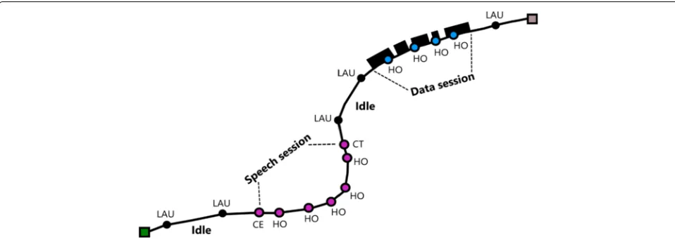
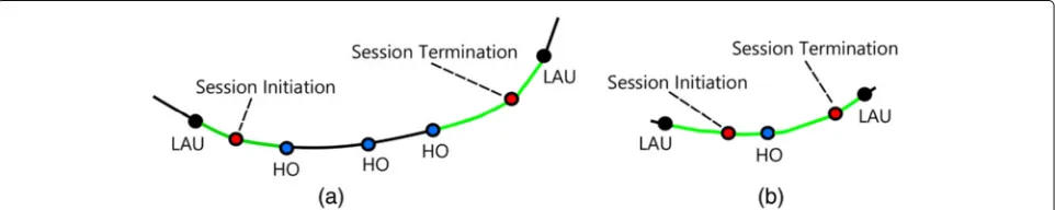
Figure 1 outlines the basic concept of our system: a tra-jectory is generated based on a given set of LAU and HO events. These events are recorded asynchronously, i.e., each event is logged on occurrence. A HO event occurs whenever the mobile terminal changes its serving cell whereas a LAU event is issued whenever a mobile terminal changes its location area. With that, we have information about the trajectory as sampling points (time-location tuples) with a certain accuracy in space domain and exact in time domain. Whilst LAU events are issued only when the subscriber is in idle mode, HO events are generated during active speech or packet data sessions. Based on the corresponding events, we can distinguish between speech and packet data sessions, which consti-tutes useful information when it comes to modeling and simulating network traffic.
We found out that trajectories can be estimated for urban as well as semi-rural environments with good accordance to the real trajectories. Our approach also allows the estimation of the subscribers’ movement veloc-ity and is therefore well-suited to describe their mobilveloc-ity.
The rest of this paper is organized as follows. In Section 2, related work in the areas of mobility model-ing, travel time estimation, and trajectory estimation is presented. In Section 3, the developed trajectory estima-tion framework is outlined. Important figures of merit and results of performed experiments and simulations are shown in Sections 4 and 5, respectively. Finally, the paper is concluded in Section 6.
2 Related work
Over the past years research has been conducted in the field of mobility simulations and investigation of mobil-ity related events in mobile communication networks. Besides mobility simulations and mobility modeling, mobile subscription data is also used for mobility behavior estimation in ITS applications. We summarize fundamen-tal concepts in all relevant areas, namely mobility mod-eling, trajectory estimations, and travel time estimations. The field of traffic modeling remains unregarded, since our work does not focus on actually modeling network traffic, but instead provides a generic solution for applying a traffic model of choice.
2.1 Mobility models
Stochastic processes are often used in order to model the human mobility behavior. The most common mobil-ity models are random way point (RWP, [1]) or random walk models (sometimes referred to as Brownian Motion, used in, e.g., [2–4]), Levy walks and flights [5, 6], and also the Gauss-Markov mobility [7]. Rhee et al. [8] com-pared the Levy walk model, which is an extended ran-dom walk model, with the human mobility, based on GPS traces of 101 volunteers. Their findings indicate that outdoor Levy walks with less than 10 km contain statistically similar features as the human mobility. To understand human mobility patterns, Gonzalez et al. [9] analyzed 100.000 anonymized trajectories of subscribers. They found out that human mobility is characterized by a time-independent travel distance and that people travel to a few highly frequented locations. In [10], the authors propose a mobility model based on the flocking behavior of birds in order to model a realistic movement of groups of mobile entities in mobile ad-hoc networks (MANETs). Similar to that Morlot et al. [11] propose an interaction-based mobility model for hot spots, i.e., their
modeling the mobility pattern of a target node in a wire-less sensor network based on available tracking data that are collected by sensing nodes. Different methods are presented to determine and predict the trajectory of the moving target node. In contrast to this work, we consider cellular systems in real environments with underlying real street networks. In [13], the authors propose a random room mobility model (RMM) in order to describe the mobility behavior of patients inside a hospital that are monitored using wireless body area networks (WBAN). With the help of this model, they studied the performance of extra-WBAN communication.
Liu et al. [14] propose a hierarchical mobility model based on user profiles which consist of a set of user mobil-ity patterns (UMPs). The model covers a global mobilmobil-ity model (GMM) and a local mobility model (LMM) in order to predict trajectories in wireless ATM networks. Whereas the GMM predicts the sequence of cells a user is moving through, the LMM determines the actual path within a cell. The sequence given by the UMP is randomly changed based on different operations (insert, delete, change). This model is somehow a random walk limited by deterministic components. Therefore, all positions within a cell are possible for the mobile. The proposed model is verified by simulations only.
2.2 Trajectory estimation
The estimation of trajectories based on mobile phone data is a topic which has been addressed by numer-ous researchers in recent years. Schlaich et al. [15] used sequences of LAUs in order to derive trajecto-ries for mobile users. Using LAUs constitutes an eligible approach, since they are issued when the mobile termi-nal is in both idle and connected mode. The ascertained sequence of LAUs is compared to a set of pre-generated routes between an estimated start and end position. In the end, the route showing the highest similarity with respect to the sequence of LAU events is chosen as the trajec-tory describing the corresponding user’s mobility. This approach works well for longer trajectories around 20 km, for short tracks however it does not work properly, since a minimum number of three LAUs is required.
Tettamanti et al. [16] used HO updates instead of LAUs, which makes their approach applicable not only for the
use in the respective areas, which can be used to deter-mine, e.g., where it is more likely that a certain trajectory starts or ends, are not taken into consideration. In order to generate different routes connecting the given start and end position, they used the traffic modeling simula-tion framework VISSIM. For each of the generated routes, the squared sum of all minimum distances between the route and the cell sites was calculated. In the end, the route with the minimal distance was chosen as the final trajectory.
Becker et al. [17] characterize the mobility pattern of hundreds of thousands of people using a huge number of anonymized call detail records (CDRs) from a cellular net-work. They characterize the human mobility in terms of daily travel distance and carbon emissions with a resolu-tion of ZIP code areas. Addiresolu-tionally they determine traffic volumes carried by different roads. For that purpose, test users drive along predefined routes and record the cor-responding sequences of cells their mobile phones are connected to. Afterwards they fit the actual cell sequence to the best predefined in order to estimate the path the user was moving along. The major difference to our work is that they distinguish only between a few predefined routes where for all of those the cell sequence has to be recorded in a training phase.
2.3 Travel time estimation
Alger et al. [18] from Vodafone Germany were one of the first who investigated travel time estimation on the German higher roads network. Double handover (DHO) events of speech users were used to compute the cell passage time, i.e., the time elapsed between entering and leaving the cell coverage area. By estimating the route a subscriber moved within the cell coverage and divid-ing it’s length by the time difference, the velocity can be computed. An average filter was used to combine the travel times of other subscribers in the same cell. The sys-tem was used to investigate the traffic condition on the higher roads network in real time. This research showed that travel times can be estimated for the higher roads network without the need of expensive inductive loop detectors. However, their approach focused only on the highway networks and does not support the minor roads network. Especially, the route estimation is very simplis-tic on highways. Since the German road network1consists of 12.917 km highway and 230.377 km other roads their approach is only applicable for 5.6 % of the entire road network.
In order to estimate the traffic speed and travel time, Bar-Gera [19] used a proprietary system developed by Estimotion Ltd. This system uses information about HO events of speech users to estimate the traveled route and velocity. A sequence of locations derived from the HO footprints is matched to road segments. Unfortunately, no information is provided about the determination of the HO footprints which are the basis for further investiga-tions.
3 Mobility estimation and traffic modeling
In this section, we give a detailed description of the methodology used in our framework. We introduce all the data that are required as input to our system as well as the algorithms to transform this data into a set of user trajec-tories. Figure 2 gives an overview of the particular steps which are performed in order to derive a users’ trajectory from a given input. The individual steps are explained in the following.
3.1 Mobile network operator data
The data described in this section are provided by the Austrian MNO A1. The MNO captures a lot of events at the interfaces of its core network by installing network probes. This process is described by Valerio [20] in detail. Each event that is captured in the core network features the following attributes:
• Timestamp: specifies the exact time when the event was captured
• ID: identifies the subscriber
• Cell ID: identifies the cell the subscriber is currently connected to
• LAC: identifies the location area the subscriber is currently assigned to
• Event: defines the type of the captured event
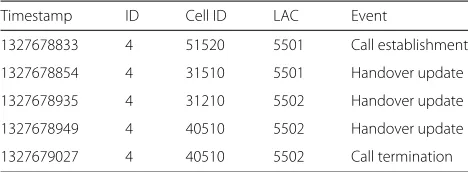
Some of these events are strongly related to the mobil-ity of the subscribers. The most important events in this respect are call establishment and termination, HO, and LAU. Each of these events can be related to a certain sub-scriber ID and the cell where the event occurred. In case of a HO event this is the cell the subscriber is handed over to (target cell), in case of a LAU event this is the target cell in the newly assigned location area. An example for a sequence of events related to a certain subscriber that was captured in the core network is depicted in Table 1. The first event describes a call establishment, followed by three HO events and a call termination event. Using the position of the involved BSs in combination with their antenna configuration (i.e., the angles of the electrical bore sight), a coarse position of the subscriber at the time the event occurred can be determined.
3.2 Road network
Based on the assumption that individuals typically move along roads, our framework maps the estimated sub-scriber trajectories on ways and streets existing in a real environment. The road network we use for that reason is obtained from OpenStreetMap. These freely available data cover a majority of the real road network and pro-vide additional information such as the maximum allowed speed on particular road segments. This information is required for adapting and validating the estimated user’s speed, whereas the road network defines the actual route of the final trajectory.
3.3 Cell area estimation
At this point, it is difficult to estimate the actual location of a particular subscriber at the time the specific event is captured as only the position of the BS the subscriber is currently connected to is known. In order to improve the estimated position, knowledge about the cell’s cover-age area (relevant for call establishment and termination events) and its borders (relevant for HO and LAU events) is inevitable. We therefore investigate two methods for determining mentioned characteristics, namely Voronoi diagrams and coverage prediction.
3.3.1 Voronoi diagrams
Fig. 2Workflow of the proposed trajectory estimation framework
Table 1Events captured in the core network of the mobile network operator A1
Timestamp ID Cell ID LAC Event
1327678833 4 51520 5501 Call establishment
1327678854 4 31510 5501 Handover update
1327678935 4 31210 5502 Handover update
1327678949 4 40510 5502 Handover update
1327679027 4 40510 5502 Call termination
x=x+cos(α) 1
50000° (1)
y=y+sin(α) 1
50000° (2)
After performing the mentioned transformations, each cell’s coverage area is described by a unique polygon, resulting from Voronoi tesselation. A subscriber located within such a polygon has the closest distance to the asso-ciated BS. Using Voronoi diagrams for cell area estimation has the advantage that every location has a well-defined affiliation to one of the BSs; moreover, the cells’ borders are defined exactly. One drawback is that eventually dif-ferent power classes of particular cells are not considered. Additionally, the influence of the BSs’ environment is also completely neglected.
3.3.2 Coverage prediction
Certain limitations of Voronoi tesselation in the scope of cell area estimation can be overcome by using pre-diction calculations through the application of network planning tools. These tools allow the incorporation of additional data, which comprises, among other things, antenna characteristics, transmitter power, and landscape characteristics.
We estimated the coverage area for all cell sites of the Austrian MNO A1 in two areas of interest. Since A1 only provided us with the location and the beam direction of its antennas, we used publicly available data sets to enrich coverage estimation. A representation of the landscape is defined by a digital elevation model2. This model offers a resolution of 25 m, which means that each pixel covers an area of 25 by 25 m. Additionally, we integrated a building block model for the two areas of interest. For the city of Linz, the footprint of every building is known from Open-StreetMap3, though, their heights is unknown. For these buildings we assumed an average height of 15 m. On the contrary, the city of Vienna4 provides a building model including height information. This model consists of the footprint of buildings and a category that specifies their heights in steps of approximately three meters.
In our building model we enriched the building lay-out from OpenStreetMap for the city of Vienna with the average height of the specified category. In total, we computed two coverage predictions for each area of inter-est. The first uses the transmitter’s location, transmitter power, and the digital elevation model. The second predic-tion enhances the first one by addipredic-tionally including the building model on top of the elevation model.
3.3.3 Transmitter power
A cell’s coverage area directly depends on the mitter power of the corresponding BS. We use trans-mitter power specifications from the Austrian Forum
Mobilkommunikation (FMK) as basis. The FMK pro-vides a service where participating MNOs can upload information about their network infrastructure. For our work the cell sites’ location and information about their transmitter power is relevant. However, there are a few limitations while using these data. First, the service pro-vided by the FMK is voluntary and therefore the data can either be out of date or even absent. Second, only the highest transmitter power of all sectors in case of a sectorized cell deployment is provided. Finally, it is not indicated which network operator a particular cell site belongs to.
In the following, our approach to retrieve transmitter power estimations for each cell site in the areas of inter-est is outlined. At first, we define two sets of locations, one for the cell sites of the provider of relevance and one for the FMK transmitters. LetA = {pos0,pos1,. . .,posi}
be a set of BS locations of the network operator andB =
{pos0,pos1,. . .,posj}be a set of BS locations provided by
the FMK. SetC = A∩Bthen contains the positions of
cell sites of the MNO of interest for which the informa-tion regarding transmitter power is available. For BSs of the same MNO where this information is not at hand (set D=A\B), an estimation is performed. Given the informa-tion (posiinforma-tions and transmitter powers) of the BSs in set C, the transmitter powers of BSs in setDare estimated by applying a scattered interpolation. An example therefore is depicted in Fig. 3. The triangles indicate the positions of BSs in set C, the transmitter power values outlined at all other positions are estimations of the transmitter power for a BS situated at the corresponding location. Different transmitter power values are depicted using dif-ferent colors, according to the color scheme shown in Fig. 3.
3.4 Start- and endpoint estimation
At this point, the framework knows the road network on which subscribers can move and the coverage area of the cell sites in the areas of interest. In order to esti-mate trajectories for a particular subscriber, we need to know where the subscriber started and ended his journey. The call establishment and termination events are used to determine those cells where the trajectory starts and ends in, respectively.
It is obvious that the probability for the location of a trajectory’s start- and endpoint is not homogeneously dis-tributed over the entire cell area. Hence, a reasonable remedy is the inclusion of land use information. In our
framework, we use the CORINE land cover5(CLC) maps
Fig. 3Transmitter power interpolation. Sample power interpolation for 20 cell sites with a random transmitter power in the range of 45–52 dBm
defines the probability that a trajectory starts or ends in an area of this kind. In this manner, the start and end position can be restricted to a few defined CLC classes such as arti-ficial surfaces, urban fabric and industrial, commercial, and transport units.
The second improvement is the use of socio-statistical maps (i.e., population density maps6). These maps are also
provided by the EEA and have the same resolution as the CORINE land cover maps. The basic assumption is that it is more likely that a trajectory starts or ends in an area with higher population density compared to other areas of the same CLC class. These maps can be used to create trajectory sets that fit better to the morning as well as to the evening hours since it is possible to incorporate the commuter traffic.
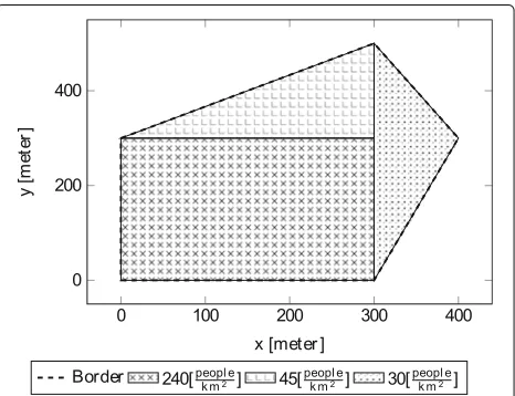
An example is depicted in Fig. 4, where a region con-sisting of three different population density areas is illus-trated. Based on our assumption the subscriber will more likely be located in the area with a population density of 240peoplekm2 rather than in those with 45
people km2 and 30
people km2 . Hence, our framework considers all different population density areas within the region’s boundaries and computes a spatial probability density function. After a population area has been selected by a random process, the exact start and end position will be selected randomly based on a uniform distribution within the bounds of the population area. In order to generate a realistic trajectory based on the underlying road network, the estimated start and end position are mapped to the closest road segment in their vicinity.
3.5 Trajectory estimation
Apart from the trajectory’s estimated start and end posi-tion, we know a series of HO and LAU events related to the locations of the corresponding BSs. Considering the estimated coverage area of every cell, a series of cells the subscriber traversed during his journey can be derived. We restrict our generated trajectories to be on top of the road network of the area of interest. In this manner, the subscriber’s route will be computed based on the Open-StreetMap road network between the estimated start and
end position. By default, 20 routes with different start and end positions will be computed. Afterwards, two plausi-bility ratings for these routes will be calculated, the first considering their geometry and the second incorporating the time it takes to traverse them.
As for the trajectory’s geometric validation, the squared sum of minimum distances between the route and the centroid of each particular cell coverage area is calculated. For each of the pre-calculated routesj, the squared sumDj
of all minimum distancesdi,jbetween the routejand cell
siteiis computed.
The second validation step verifies the trajectories with respect to the time required to traverse them. For this pur-pose, we introduce a duration ratiorouteratiobetween the
call or packet session durationtsessionand the time it takes
to traverse the routetroute, as depicted in Eq. (4). This
met-ric provides information whether the estimated route is either too short or too long.
routeratio=
tsession
troute
(4)
The squared sumDj in combination with the duration
ratiorouteratio is used to select the most likely route the
subscriber has traveled with respect to the distance to involved cell sites and ascertained travel time. More pre-cisely, the route which is showing a minimal Dj and a
routeratiowhich is closest to or equal to 1 is selected as the
subscriber’s trajectory.
3.6 Velocity estimation
The average velocity of a moving subscriber between two successive HO or LAU events can be calculated by sim-ply dividing the distance on the road network between the two event locations by the passage time (difference of the two timestamps). Very accurate timestamps are available from the MNO data, whereas the estimation of the actual HO and LAU event positions needs a closer look.
3.6.1 Handover position
HO events in cellular networks are usually initiated if the network decides that the serving cell of a mobile terminal is no longer the best available cell. The best serving cell is typically the one that guarantees the aspired quality-of-service (QoS) with the least necessary transmitter power. Therefore, the position where a HO is executed correlates with the coverage areas of the two involved cells. In reality, the coverage areas of neighboring cells overlap in order to guarantee a seamless HO. Two aforementioned methods to determine the coverage area of a cell are used in our framework.
When using Voronoi diagrams, every cell has a well-defined and unique coverage area, i.e., no overlapping or gap between the coverage areas of two neighboring cells can occur. Since the HO can only take place on the trajec-tory the intercept between this trajectrajec-tory and the border between the involved cells is the estimated position of the HO event.
Using the coverage prediction method, we have to deal with three different situations concerning the estimated coverage areas of the involved cells,
1. Overlapping handover: The estimated coverage areas of the two involved cells intersect with each other (see Fig. 5a).
2. Unconnected handover: The estimated coverage areas of the two involved cells do not intersect (see Fig. 5b). This means that a HO is made to a cell site whose coverage area the subscriber has not entered yet. Although such situations are very unlikely in reality we sometimes have to deal with them. This is because our input data for the coverage prediction are not as complete as they should be. It would require additional knowledge of used antenna configurations and transmission power to estimate the coverage area of the concerned cell sites more precisely. As we are using only freely available data sources, we lack this kind of information.
3. Ping-pong handover: A HO is performed from cell A to cell B and later back to A although the trajectory does not contain lines that are used twice. These HOs are an undesirable effect not only for the network itself but also for the timing estimation. Therefore, we filtered out ping-pong HOs by removing the last HO event, in this specific case the HO event from B to A.
Algorithm 1 depicts how the system estimates the HO position for the overlapping and the unconnected HO type. For an overlapping HO the centroid of the
inter-section C = A ∩B of the involved cells is computed
and mapped onto the calculated trajectory. For an uncon-nected HO, the line between the closest points of the two coverage areas is computed. If this line intersects the previously computed route then the point of inter-section is set as the HO position. If this is not the case then the midpoint of the line is mapped onto the route.
3.6.2 Location area update position
Fig. 5Different types of handover. An overlapping handover (a) and an unconnected handover (b) are depicted together with the estimated handover position (red point)
Algorithm 1Handover prediction 1: HP←List()
2: fori←1 tolength(handover)−1do 3: cur=handover[i]
4: next=handover[i+1] 5: ifIntersects(cur,next)then
6: centroid=Centroid(Intersects(cur,next)) 7: Add(HP,NearestPoint(route,centroid)) 8: else
9: line=LineBetweenNearestPoint(cur,next) 10: ifIntersects(line,route)then
11: Add(HP,Intersects(line,route)) 12: else
13: midPoint=MidPoint(line)
14: Add(HP,NearestPoint(route,midPoint)) 15: end if
16: end if
17: end for
for the particular LAU events. The derivation procedure however differs slightly and will be outlined hereinafter.
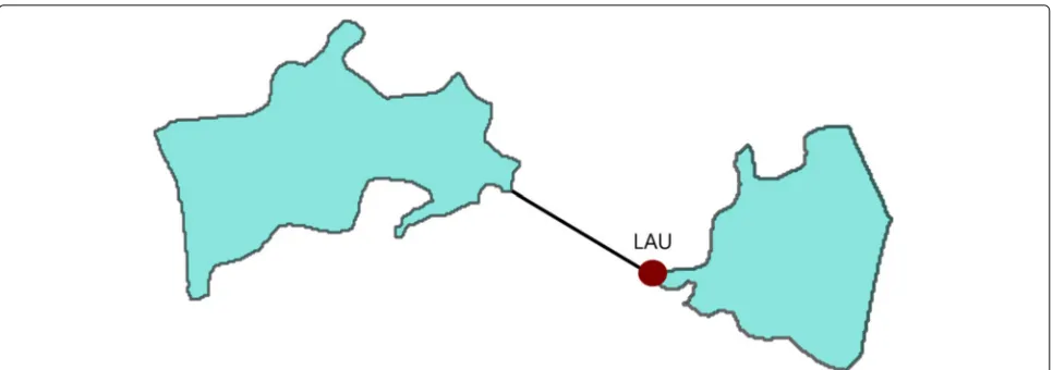
The first step is similar to what is done when dealing with an unconnected HO, which means that a line con-necting the two closest points of both coverage areas is computed. In contrary, the end point of the line which is located closest to the cell site where the actual LAU event was issued is presumed to be the most reasonable posi-tion for the corresponding event (Fig. 6). This is due to the fact that LAUs occur in close proximity to the cell site in which the event was actually triggered (based on the avail-able network data). The same applies if the two coverage areas are overlapping, in this case the closest point of the intersection area is chosen to be the location where the event was issued.
3.6.3 Average velocity
After the HO and LAU positions have been estimated, the average velocity of the subscriber between two consecu-tive event locations can be computed. Each event exhibits
a timestamp which indicates when the event occurred. In order to derive the subscriber’s velocity, the distance on the road network between two event positions is divided by the difference of their timestamps.
3.6.4 Velocity adaption
Whilst the timestamps of HO and LAU events are very precise, the estimated positions are not. This can yield in completely unrealistic average velocities between two suc-cessive estimated event positions. If the distance between two events is estimated as too long, the estimated average velocity can be much higher than the maximum allowed speed on that particular road. Since the speed limit is known for each street segment from OpenStreetMap data, this information can be used to adapt the estimated event positions in order to obtain realistic velocities (see Algorithm 2).
First of all, the trajectory is partitioned into so-called event segments, which represent the partial trajectories connecting two successive HO or LAU positions. Each of these segments is verified with respect to its con-formance with the average velocity and the maximum allowed speed on the respective road segments. If the average speed exceeds the allowed limit by a certain fac-tor (we decided to permit a maximum velocity of 1.7 times the allowed speed limit, this factor however can be chosen on demand), the afflicted HO or LAU event positions are repositioned. This is done by moving the respective posi-tions back and forth along the trajectory. By increasing or decreasing the distance between two event positions, the afflicted segments’ average velocity will be altered in the same way.
Fig. 6Location area update position. Estimating the position of a location area update event based on two cell coverage areas. Theright cellis the cell where the event was issued, theleft cellis the one where the subscriber was connected to previously
Algorithm 2Handover adaption
1: fori←2 tolength(trajectory)−1do
2: allowedSpeed=MaxSpeed(trajectory[i]) 3: cur=trajectory[i]
4: prev=trajectory[i−1] 5: next=trajectory[i+1] 6:
7: ifSpeed(cur)≥1.7∗allowedSpeedthen 8: curDist=Distance(cur)
9: prevDist=Distance(prev) 10: nextDist=Distance(next)
11: nominalDist=allowedSpeed∗Duration(cur) 12: SetSpeed(cur,allowedSpeed);
13:
14: nextTempDist = nextDist + (curDist −
nominalDist)/2
15: prevTempDist = prevDist + (curDist −
nominalDist)/2 16:
17: if nextTempDist/Duration(next)
nominalSpeedthen
18: nextTempDist=nextDist
19: prevTempDist = prevDist + (curDist −
nominalDist)
20: else if prevTempDist/Duration(prev) nominalSpeedthen
21: nextTempDist = nextDist + (curDist −
nominalDist)
22: prevTempDist=prevDist
23: end if
24:
25: SetSpeed(next,nextTempSpeed/Duration(next)) 26: SetSpeed(prev,orevTempSpeed/Duration(prev)) 27: end if
28: end for
displacement of particular positions however also affects the previous and/or the subsequent event segments. This implies that for certain segments only the first, the last, or both event positions have to be displaced in order to guar-antee realistic velocities in the adjacent segments. In this manner, the entire trajectory is traversed.
3.7 Traffic model framing
As mentioned in the beginning, MNOs capture various kinds of events in their core network that allow to deduce, e.g., if a particular mobile terminal is in idle or connected mode or his coarse position at cell coverage level. Fur-thermore, these events can be used to distinguish between speech and data users, as different events are issued for the respective connection types. These HO events (or LAU events in case the mobile terminal is in idle mode) can be used in order to infer the subscriber’s mobility behav-ior in terms of a movement trajectory, as outlined in the previous sections. For the reason of reproducible mobility situations in cellular real-network simulations at system level, the modeling and simulation of network traffic is an important aspect. In our work we do not focus on particular traffic models (examples are given in [22–24]); instead, we offer a generic solution that allows to estimate when a speech or data session started and ended, both in a time, and spatial dimension. The actual traffic model to be applied at a later point in time is freely selectable, which adds additional flexibility to the simulations to be performed.
or termination events are issued as it is the case for speech users. On that account, we assume that a packet data ses-sion starts somewhere between the last LAU and the first related HO event. The same applies for the termination of the session, just the other way round. For estimating the position when a particular data session starts or ends, we use a uniformly distributed random variable in order to obtain the definite estimation of the location of the par-ticular event. Figure 7 outlines this concept based on two simple scenarios.
4 Figures of merit
In order to evaluate our findings, we make use of a number of metrics that allow us to assess the estimated trajec-tories with respect to the ground truth trajectory, which was recorded using a GPS tracker. The first part of the evaluation affects the estimated route of the trajectory, which is compared to the actual one in order to derive a similarity factor. Secondly, the estimated HO positions are confronted with the real ones. For that reason, a mobile terminal was used during test rides in order to record the exact position where the moving subscriber was handed over to a new cell site or location area. Finally, the estimated velocities are verified using the recorded GPS tracks. Hereinafter, the used metrics are described in more detail.
4.1 Route geometry
In order to evaluate the estimated trajectory with respect to the actual, recorded one, we use two different metrics,
distances from a pointx in subset X to the closest pointy in subset Y. In Eq. (5), X and Y are the sets representing all pointsx of the estimated and all pointsy of the actual route, respectively, d(x,y) constitutes the distance between a pointx and a pointy.
dH(X,Y)=max
sup
x∈X
inf
y∈Yd(x,y), supy∈Yxinf∈Xd(x,y)
(5)
2. TheFréchet distance constitutes a measure of similarity between curves, which takes the actual position and order of points along the curves into consideration. We consider the algorithm developed by Alt and Godau [26] which computes the Fréchet distance of two polygonal curves in Euclidean space. Hence, the Fréchet distance for two curves
A,B:[ 0, 1]→V, in our case two routes, is defined as
δF(f,g)= inf
α[0,1]→[a,a]
β[0,1]→[b,b]
max
t∈[0,1]f(α(t))−g(β(t))
(6)
whereαandβare continuous functions with α(0)=a,α(1)=a,β(0)=bandβ(1)=b. Our evaluation was done using Christophe Genolinis’ implementation of the Fréchet distance [27].
4.2 Handover deviation
Since we estimate the HO and LAU position based on the geometry of the coverage area of the involved cell sites, we need a metric that indicates how far the estimated posi-tions deviate from the observed ground truth posiposi-tions. The Euclidean distanced(x,y)(in two-dimensional space, Eq. (7)) between the estimated positionx = (x1,x2)and
the observed oney = (y1,y2)is used as a metric. It is
the basis to evaluate the position prediction as well as the coverage area estimation.
d(x,y)=
(y1−x1)2+(y2−x2)2 (7)
4.3 Velocity comparison
In order to verify our approach, we compare the esti-mated and adapted (refer to Algorithm 2) velocity with the ground truth velocity which can be obtained from recorded GPS information.
One of the metrics we use for this reason is themean absolute error(MAE, Eq. (8)) between the observed aver-age velocityviand the computed velocityvˆi. The observed
average velocity vi is the velocity obtained from GPS
between the two successive HO positions. The computed velocity is derived by calculating the distance between the successive HO locations divided by the time difference between the corresponding events.
The second metric is theroot mean square error(RMSE, Eq. (9)), which is stronger influenced by large errors than by small ones. In both equations the variablenrepresents the number of event segments a trajectory consists of.
RMSE=
In this section, we present results which have been achieved using the described methodology. For the rea-son of evaluation, we performed test drives in urban and semi-rural areas in Upper Austria and the city of Vienna. The recorded data are used as a reference in order to validate the estimated subscriber trajectories. First of all, we characterize the test setup and the test environment. Subsequently, we present various metrics and figures that allow to quantify the achieved results with respect to actual data. We show that our approach constitutes an eligible method to derive realistic trajectories for sub-scribers in a cellular network in both urban and semi-rural environments.
5.1 Environment
As mentioned beforehand, we performed several test drives in order to capture data which is required to verify our approach towards trajectory estimation. For each of these test drives, we were using the identical mobile termi-nal with the same subscriber identity module (SIM). The handset in use was a Samsung S3 running the Android 4.1.1 JellyBean operating system. During the test drives, the handset was used to initiate speech and data sessions. Throughout the entire drives, the mobile terminal’s cur-rent position was recorded using a GPS tracker. Additional information regarding the actual serving cell sites and location areas was logged in order to derive the effective position of potential HO or LAU events. At a later time, the Austrian MNO A1 provided us with the subscriber information and events captured in the core network for the particular test drives. These data were used to derive the subscriber’s trajectory, whereas the recorded data was required for validation and quantification.
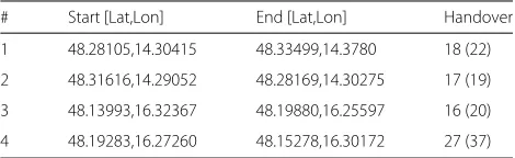
Table 2 gives an overview of the start and end position and the number of HO events for each of the performed test drives. The number of HOs in brackets corresponds to the unfiltered raw events captured by the core net-work, the second number represents the same set of HO events after removing ping-pong HOs. The first test drive started in the city of Linz and ended in Treffling, a small town in the outskirts of Linz. This test drive was per-formed entirely on the higher road network and features a semi-rural scenario that consists of an urban and a rural section (trajectory depicted in Fig. 8). The second test drive took place within the borders of the city of Linz. This drive was performed on streets of the minor road network as well as on the city highway. The third and fourth test drive (refer to Fig. 9) took place in the city of Vienna. Both test drives were performed on the major and minor road network and constitute an urban mobility scenario.
5.2 Results
In order to be able to quantify and rate the devel-oped mechanisms and procedures, evaluating the results achieved using our system with actual data is inevitable. For that reason, all in all, four test drives in different
Table 2Overview of the start and end position and the number of HO events for the four test drive trajectories
# Start [Lat,Lon] End [Lat,Lon] Handover
1 48.28105,14.30415 48.33499,14.3780 18 (22)
2 48.31616,14.29052 48.28169,14.30275 17 (19)
3 48.13993,16.32367 48.19880,16.25597 16 (20)
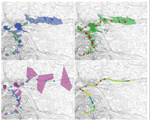
Fig. 8Trajectory 1. Estimation of event positions based on different coverage prediction methods: Coverage prediction (top left), coverage prediction including height and building model (top right) and Voronoi tessellation (bottom left). The last picture shows the original trajectory recorded using a GPS tracker (black) and the estimated trajectory based on event positions derived from the top right image (green). Thepurple pointsindicate an active speech session, the blue ones a data session, respectively. Theyellow pointsare the actual event positions which have been recorded using a handset
environments have been performed in order to collect reference data. This data basis allows to verify the esti-mated trajectories using real data under different aspects. First of all, the route geometries of the estimated trajec-tory and the actual one are confronted, and a similarity factor is derived. Furthermore, the deviation of the effec-tive HO positions and the estimated ones is computed. The last evaluation aspect covers velocity estimation, which is done by comparing the derived subscriber veloc-ity with the ground truth recorded by a GPS tracker. The findings presented on the following pages indicate that our approach constitutes an appropriate method for deriving subscriber trajectories based on mobile network operator data.
5.2.1 Route geometry
Fig. 9Trajectory 4. Estimation of event positions based on different coverage prediction methods: Coverage prediction (top left), coverage prediction including height and building model (top right) and Voronoi tessellation (bottom left). The last picture shows the original trajectory recorded using a GPS tracker (black) and the estimated trajectory based on event positions derived from the top right image (green). Thepurple pointsindicate an active speech session, the blue ones a data session, respectively. Theyellow pointsare the actual event positions which have been recorded using a handset
0.0012°(94 m) and 0.0047°(370 m), respectively intimate a high similarity between the actual and the estimated trajectory for all four test cases.
5.2.2 Handover deviation
In order to verify the performance of our HO position-ing algorithm, we compare three differently estimated HO
Table 3Route similarity computed with the discrete Hausdorff distance and the Fréchet distance
Trajectory dH(X,Y) δF(f,g)
1 0.0135° 0.0047°
2 0.0075° 0.0015°
3 0.0151° 0.0021°
4 0.0107° 0.0012°
positions—each of them using a specific coverage esti-mation method—with the actual positions recorded by a mobile terminal.
indicate the three different coverage estimation methods. It can be seen that the deviation increased in the second half of the plot. This was caused by leaving the urban area and driving into a semi-rural one. Here, Voronoi diagrams performed worse compared to the other coverage predic-tions. The reason for this is that in rural environments the cell coverage areas get larger and the differences between Voronoi polygons and real coverage areas increase since Voronoi tesselation does not consider any terrain informa-tion. On the other coverage prediction hand is able to take such environmental information into account. This in fur-ther consequence leads to smaller errors in estimating HO positions.
Table 4 shows the minimum, the first quartile, the median, the mean, the third quartile and the maxi-mum position deviation in kilometers for all four test
2 PB 0.132 0.261 0.346 0.399 0.525 0.884
2 V 0.048 0.229 0.343 0.386 0.482 0.900
3 P 0.111 0.360 0.449 0.677 0.604 3.786
3 PB 0.148 0.338 0.451 0.679 0.536 4.062
3 V 0.013 0.281 0.409 0.669 0.639 4.085
4 P 0.020 0.223 0.309 0.355 0.504 0.863
4 PB 0.030 0.213 0.325 0.359 0.506 0.850
4 V 0.010 0.175 0.321 0.328 0.443 0.802
trajectories. All HO positions have been estimated with Algorithm 1 and were performed with the three men-tioned coverage estimation methods.
By combining the HO deviations over all four test tra-jectories and computing the MAE and RMSE, coverage
prediction without building information performed best with a MAE of 0.176 km and a RMSE 0.231 km, fol-lowed by the extended coverage prediction with a MAE 0.189 km and a RMSE 0.253 km and Voronoi diagrams with a MAE 0.238 km and RMSE 0.311 km. The slightly higher errors when using coverage prediction including a building model originate from the inaccurate building heights, which are either completely unknown (e.g., city of Linz, where an average height of 15 m is assumed) or available in an inadequate resolution (e.g., city of Vienna). For the fourth trajectory in particular the minimum, maximum and mean HO position deviations are 0.010, 0.802, and 0.328 km, respectively, which shows that the HO positions can be estimated with high accuracy.
The third trajectory shows a high maximum HO devi-ation which was caused by the network not performing a HO while driving for 3.55 km within the city of Vienna. Since the HO algorithm computed a HO position between the two cell site coverage, areas that were far-off a large HO deviation occurred.
5.2.3 Velocity estimation
In this section, we want to discuss the results of the raw velocity estimation and the adapted velocity estimation after HO repositioning. We compared each of the veloc-ities against the ground truth velocity derived from the
recorded GPS data. Since the estimated velocity accords to the average velocity between two HO positions we com-puted the average GPS velocity between the respective HO positions. In Fig. 11, the raw estimated velocity for the first trajectory is illustrated. It can be seen that there occur many velocity overruns for all coverage estimation methods. By comparing this figure with the HO deviation (see Fig. 10) it becomes obvious that a velocity overrun is caused by a large deviation between the estimated and the actual HO position (≥0.5 km).
In contrast, Fig. 12 depicts the estimated velocity after applying the adaption and HO repositioning algo-rithm. Hence, we see that the bigger deflections could be reduced. To verify the accuracy of the estimated veloc-ity, the MAE and RMSE for both velocity estimations and for each trajectory and coverage prediction method were computed. The results are shown in Table 5 and indicate that the adaption algorithm can reduce the error intro-duced by a wrong HO position estimation significantly.
For the coverage prediction without building model, the velocity MAE using the adaption algorithm was reduced on each trajectory by an average of 60.40 %. For the coverage prediction enhanced with a building model the reduction was 65.75 %, for Voronoi diagrams 73.01 %.
However, this indicates only how well the adaption algo-rithm works but not how accurate the velocity estimation
Fig. 12Velocity estimation with adaption. The estimated velocity for all three coverage estimation methods after applying the adaption algorithm
is in general. To validate this for the three different cov-erage prediction methods, the absolute adapted veloc-ity errors from the four trajectories were combined in order to compute the MAE. Here, the coverage prediction enhanced with a building model had the minimum abso-lute error for all trajectories with 14.887 km/h, followed by Voronoi diagrams with 14.921 km/h and coverage predic-tion without building model 16.004 km/h. This indicates
Table 5MAE and RMSE for the four test drive trajectories using three different coverage predictions
# M MAE RMSE MAEadpated RMSEadapted
1 P 42.365 62.593 23.360 31.514
1 PB 50.315 69.985 23.127 29.142
1 V 59.704 85.549 17.648 25.250
2 P 81.304 138.707 8.970 16.047
2 PB 60.964 99.090 9.436 12.086
2 V 113.999 181.854 13.029 16.932
3 P 21.125 26.808 13.305 17.799
3 PB 26.384 33.786 11.941 16.607
3 V 28.449 40.088 13.036 18.781
4 P 58.425 150.199 17.081 22.000
4 PB 48.061 125.747 14.553 17.795
4 V 72.715 191.037 15.388 21.599
that post-processing using the adaption algorithm is nec-essary in order to estimate an accurate movement velocity for a particular subscriber.
6 Conclusions
The presented results show that cellular network sub-scriber trajectories can be generated for the purpose of mobility simulations. These trajectories cover the sub-scriber’s route and provide its velocity and are therefore well-suited to describe the subscriber’s mobility behavior. Furthermore, based on the estimated position of the cor-responding HO and LAU events, it is possible to derive a time and spatial frame for applying a traffic model for a single subscriber, which is useful, e.g., for real network traffic simulations.
Endnotes
1Statistics about the German road network [28].
2The Digital Elevation Model over Europe from the
GMES RDA project: http://www.eea.europa.eu/data-and-maps/data/eu-dem.
3More information about how building information
can be retrieved from OpenStreetMap: http://wiki. openstreetmap.org/w/index.php?title=Buildings&oldid= 1050850.
4The GIS service of the city of Vienna: https://www.
wien.gv.at/kultur/kulturgut/architektur/gebaeudedaten. html.
5Corine Land Cover 2006 seamless vector data: http://
www.eea.europa.eu/data-and-maps/data/clc-2006-vector-data-version-3.
6Population density disaggregated with Corine land
cover 2000: http://www.eea.europa.eu/data-and-maps/ data/population-density-disaggregated-with-corine-land-cover-2000-2.
Acknowledgements
This project was supported by the program Regionale Wettbewerbsfähigkeit OÖ 2010-2013, which is financed by the European Regional Development Fund and the Government of Upper Austria.
Competing interests
The authors declare that they have no competing interests.
Received: 18 January 2015 Accepted: 27 June 2016
References
1. J Broch, DA Maltz, DB Johnson, Y-C Hu, J Jetcheva, inProceedings of the 4th Annual ACM/IEEE International Conference on Mobile Computing and Networking. A performance comparison of multi-hop wireless ad hoc network routing protocols, MobiCom ’98 (ACM, New York, 1998), pp. 85–97
2. I Rubin, CW Choi, Impact of the location area structure on the performance of signaling channels in wireless cellular networks. Comm. Mag.35(2), 108–115 (1997)
3. JJ Garcia-Luna-Aceves, EL Madrga, inProceedings of the Joint Conference of the IEEE Computer and Communications Societies (INFOCOM). A multicast routing protocol for ad-hoc networks (IEEE, New York, 1999), pp. 784–792 4. MM Zonoozi, P Dassanayake, User mobility modeling and characterization of mobility patterns. IEEE J. Sel. Areas Commun.15(7), 1239–1252 (2006)
5. BB Mandelbrot,The Fractal Geometry of Nature. (W.H. Freeman and Company, New York, 1982)
6. MF Shlesinger, GM Zaslavsky, J Klafter, Strange kinetics. Nature.163, 31–37 (1993)
7. B Liang, ZJ Haas, inProceedings of IEEE Information Communications Conference (INFOCOM 1999). Predictive distance-based mobility management for pcs networks (IEEE, New York, 1999), pp. 1377–1384 8. I Rhee, M Shin, S Hong, K Lee, SJ Kim, S Chong, On the Levy-walk nature of
human mobility. IEEE/ACM Trans. Networking.19(3), 630–643 (2011) 9. MC Gonzalez, CA Hidalgo, A-L Barabasi, Understanding individual human
mobility patterns. Nature.453(7196), 779–782 (2008)
10. S Misra, P Agarwal, Bio-inspired group mobility model for mobile ad hoc networks based on bird-flocking behavior. Soft. Comput.16(3), 437–450 (2012)
11. F Morlot, I École, N Supérieure, F Baccelli, SE Elayoubi, inProceedings of IEEE INFOCOM. An interaction-based mobility model for dynamic hot spot analysis (IEEE, New York, 2010), pp. 1–9
12. S Misra, S Singh, M Khatua, MS Obaidat, Extracting mobility pattern from target trajectory in wireless sensor networks. Int. J. Commun. Syst.28(2), 213–230 (2015)
13. S Misra, J Mahapatro, M Mahadevappa, N Islam, Random room mobility model and extra-wireless body area network communication in hospital buildings. IET Networks.4(1), 54–64 (2015)
14. T Liu, P Bahl, I Chlamtac, Mobility modeling, location tracking, and trajectory prediction in wireless atm networks. IEEE J. Sel. Areas Commun. 16(6), 922–936 (2006)
15. J Schlaich, T Otterstätter, M Friedrich, inProceedings of the 89th Annual Meeting Compendium of Papers. Generating Trajectories from Mobile Phone Data (Transportation Research Board of the National Academies, Washington D.C., 2010)
16. T Tettamanti, H Demeter, V István, Route choice estimation based on cellular signaling data. Acta Polytechnica Hungarica.9(4), 207–220 (2012) 17. R Becker, R Cáceres, K Hanson, S Isaacman, JM Loh, M Martonosi, J Rowland,
S Urbanek, A Varshavsky, C Volinsky, Human mobility characterization from cellular network data. Commun. ACM.56(1), 74–82 (2013)
18. M Alger, E Wilson, T Gould, R Whittaker, N Radulovic, Real-time Traffic Monitoring using Mobile Phone Data (2004). http://www.maths-in-industry.org/miis/30/. Accessed 12 Jan 2015
19. H Bar Gera, Evaluation of a cellular phone-based system for
measurements of traffic speeds and travel times: a case study from Israel. Transp. Res. C.15(6), 380–391 (2007)
20. D Valerio, Road Traffic Information from cellular network signaling. Technical Report FTW-TR-2009-003 (2009)
21. A-E Baert, Semé, inInternational Symposium on Algorithms, Models and Tools for Parallel Computing in Heterogenous Networks. Voronoi Mobile Cellular Networks: Topological Properties (IEEE Computer Society, Los Alamitos, 2004), pp. 29–35
22. 3rd Generation Partnership Project 2, CDMA2000 Evaluation Methodology, Revision A (2009). http://www.3gpp2.org/public_html/ specs/C.R1002-A_v1.0_Evaluation_Methodology.pdf. Accessed 12 Jan 2015 23. European Telecommunications Standards Institute, Universal Mobile
Telecommunications System (UMTS): Selection Procedures for the Choice of Radio Transmission Technologies of the UMTS (UMTS 30.03 version 3.2.0) (1998). http://www.etsi.org/deliver/etsi_tr/101100_101199/101112/ 03.02.00_60/tr_101112v030200p.pdf. Accessed 12 Jan 2015
24. ND Tripathi, inVehicular Technology Conference, 2001. VTC 2001 Fall. IEEE VTS 54th. Simulation based Analysis of the Radio Interface Performance of an IS-2000 System for various Data Services, vol. 4 (IEEE, Atlantic City, 2001), pp. 2665–2669
25. F Hausdorff,Grundzüge der Mengenlehre. (Veit and Company, Leipzig, 1914) 26. H Alt, M Godau, Computing the Fréchet distance between two polygonal
curves. Int. J. Comput. Geom. Appl.5, 75–91 (1995)
27. C Genolini, Computing the Fréchet Distance between two Trajectories (2014). https://cran.r-project.org/web/packages/longitudinalData/ longitudinalData.pdf. Accessed 14 Sept 2016