Design of Packet Based Block Codes with Shift Operators

Volume 2010, Article ID 263210,12pages doi:10.1155/2010/263210

Research Article

Design of Packet-Based Block Codes with Shift Operators

Ali Al-Shaikhi

_{and Jacek Ilow}

1_{Department of Electrical Engineering, King Fahd University of Petroleum and Minerals, P.O. Box 1203, Dhahran 31261, Saudi Arabia} 2_{Department of Electrical and Computer Engineering, Dalhousie University, 1360 Barrington St., P.O. Box 1000 Halifax,}

NS, Canada B3J-2X4

Correspondence should be addressed to Ali Al-Shaikhi,[email protected]

Received 22 October 2009; Accepted 31 December 2009

Academic Editor: Nicholas Kolokotronis

Copyright © 2010 A. Al-Shaikhi and J. Ilow. This is an open access article distributed under the Creative Commons Attribution License, which permits unrestricted use, distribution, and reproduction in any medium, provided the original work is properly cited.

This paper introduces packet-oriented block codes for the recovery of lost packets and the correction of an erroneous single packet. Specifically, a family of systematic codes is proposed, based on a Vandermonde matrix applied to a group ofkinformation packets to constructrredundant packets, where the elements of the Vandermonde matrix are bit-level right arithmetic shift operators. The code design is applicable to packets of any size, provided that the packets within a block ofkinformation packets are of uniform length. In order to decrease the overhead associated with packet padding using shift operators, non-Vandermonde matrices are also proposed for designing packet-oriented block codes. An efficient matrix inversion procedure for the off-line design of the decoding algorithm is presented to recover lost packets. The error correction capability of the design is investigated as well. The decoding algorithm, based on syndrome decoding, to correct a single erroneous packet in a group ofn=k+rreceived packets is presented. The paper is equipped with examples of codes using different parameters. The code designs and their performance are tested using Monte Carlo simulations; the results obtained exhibit good agreement with the corresponding theoretical results.

1. Introduction

Real-time applications are delay sensitive and, in the Internet, are primarily based on user datagram protocol (UDP). Packet-level forward error correction (FEC) is a packet loss recovery technique which does not require retransmissions and allows packet delivery with bounded delay and

con-trollable reliability [1]. In order to protect k information

packets, r = n−k additional redundancy packets are also

sent. The term “packet” is loosely applied in this context, as in many proposals, packet-level FEC is used at the data-link layer. Packet-level FEC aims at recovering some of the lost packets, where the lost packets originate from erroneous bit transmissions and packet discarding at the lower protocol layers, especially for multihop networks, as well as from

congestions in the network and buffer overflows. When

packet level FEC is deployed alone to recover from lost packets, the packet loss rate (PLR) is reduced compared to the PLR in the network. However, there is no guarantee that all packets will be recovered at the destination. This is acceptable in some applications like video and audio

streaming or multicasting protocols [2].

The parity packets in the existing packet-level FEC schemes are constructed in a similar fashion as parity bits/symbols in the linear block codes used in digital transmission systems, except the bits used in the encoding

process are from different packets. The receiver is able to

recover up to a certain number of lost/erroneous packets in

a block ofntransmitted packets governed by the minimum

distance of the code [1,3].

There are a number of powerful and efficient FEC

schemes to recover from erasures and/or errors [4], such

as low density parity check (LDPC) codes and tornado

codes, which use bipartite graphs [2,5]. Also, Reed Solomon

(R-S) codes are used in many applications. However, the codewords in these codes are rather short, and this dictates the construction of the parity packets, which are usually visualized as arranging information packets row-wise and

running the FEC code column-wise [6, 7]. An alternative

to this is to use the turbo codes to construct the turbo code frame, and then split the frame into packets. This is only feasible in turbo codes because of the large size of the

In practical applications, in addition to erasure/error recovery capability of the code, another important aspect to consider is the complexity of the encoding and decoding

processes [9]. This aspect motivates the investigations in this

paper, where the only operations permitted on packets are arithmetic packet shifts and binary additions. Particularly,

this paper focuses on systematic codes with coefficient

matrices based on the Vandermonde or NonVandermonde structures. Both designs, by incorporating packet shifts,

facil-itate fast matrix-vector multiplication and efficient inversion

of submatrices involved in the erasure or erroneous packet recovery processes. In contrast to other systematic erasure codes based on Vandermonde matrices, the proposed codes are not using Vandermonde matrices to manipulate elements (packet fragments) from the Galois field (GF), but rather use them to operate on whole packets by working with their shifts. The benefit of this approach is the lower encoding and decoding complexities of the designs presented in this paper. The proposed codes are maximum distance separable (MDS) and, while maintaining comparable performance as in the more conventional ones, are also quite flexible in the choice of the code rate.

2. Linear Block Codes in Packet-Level FEC

In conventional applications of systematic codes to

packet-level FEC, a unit of information, either symbol or bit,mi,

i = 1,. . .,k, is taken from each of the k information

packets. These k symbols are used to construct r parity

symbols with the help of the coefficient matrixP. The parity

symbols are then transmitted inrredundancy packets. The

coded/transmitted symbols onn=r+kpackets, represented

by the column vector p, are calculated at the transmitter

(encoder) using the following linear system of equations:

G·m=p, (1)

wheremis the column vector ofkinformation symbols from

k packets, G =

_I

···

P

is then×k generator matrix, and

I is the k×k identity matrix. For R-S codes, the matrix

multiplication in (1) uses GF arithmetics. In general, if all

information packets are of the same length L, (1) is used

L/b+ 1 times to construct the coded packets, wherebis

the number of bits represented in each symbol and· is

the floor operator. The assumption used in this paper is that all packets in the coded group are of the same length. This imposes some limitations which can be overcome by padding the packets to the same length. For brevity of notation, for

all symbols in the group of packets, we rewrite (1) using the

packet version of this relationship as:

G·M=P, (2)

where M is a matrix of information packets arranged in

rows, each with L/b+ 1 symbol elements, and P is the

corresponding matrix of coded packets.

At the receiver side, for MDS codes, if there are lost information packets, we have to solve the following system

of equations forM:

Gk·M=Pk (3)

or equivalently, determine

M=Gk−1_·Pk_{, (4)}

wherePk_{is the vector of anykreceived packets,G}k_{is ak×k}

submatrix ofGwith rows corresponding to thek received

packets as determined by the received packets sequence

numbers, and (·)−1represents the inverse of a matrix. There

are many matrix inversion techniques that could be used, such as those based on Cramer’s rule procedure, Gaussian

elimination, or Gaussian Jordan elimination methods [10–

12]. We will present later a suitable technique for our designs

for finding the matrix inverse efficiently for the proposed

codes.

The main challenge in the design of an erasure code

is to determine G, or in the case of systematic codes, the

corresponding coefficient matrix P. For MDS codes, the

matrixGshould be designed in such a way that anyk×k

submatrix, Gk_{, has to be invertible (full rank). The total}

number of such submatrices isn_k, where ·_·represents

then-choose-koperator. The simplest two designs ofGare

the repetition code and the single parity check code. In the

former case, the code is (n, 1,n) wherePis the column vector

of all 1’s, while the latter is the code (k + 1,k, 2) which

adds one more packet consisting of the parity check of all

information packets; that is,P is the row vector of all 1’s.

These two codes, though simple to use, are not the best, since the former has a low rate while the latter recovers at most only one missing packet. In the case of the systematic codes considered in this paper, there are other matrices that could

be used asPresulting in the desired properties ofGk_being

invertible, such as the Cauchy and Vandermonde matrices. We will discuss next the Vandermonde matrix which is used

as the coefficient matrix P in the R-S erasure codes. The

Vandermonde matrix is also utilized in the design of the

proposed code in this paper, but with a different building

element than in the case of R-S codes.

The Vandermonde matrixV, withr×kelements, is given

by the following [13]:

V=

⎡ ⎢ ⎢ ⎢ ⎢ ⎢ ⎢ ⎢ ⎢ ⎢ ⎢ ⎣

1 α0 α20 · · · αk0−1 1 α1 α21 · · · αk1−1 1 α2 α22 · · · αk2−1

..

. ... ... . .. ...

1 αr−1 α2r−1 · · · αkr−−11 ⎤ ⎥ ⎥ ⎥ ⎥ ⎥ ⎥ ⎥ ⎥ ⎥ ⎥ ⎦

. (5)

This matrix is proven to be nonsingular if the parameters

αz, for z = 0,. . .,r − 1, are distinct. For R-S erasure

codes with P = V, the αz elements are taken from the

extended GF, GF(pb_{), where p is a prime number (p = 2}

used for highest efficiency to represent a byte). Therefore,

multiplication and addition operations in (2) and in (4)

must be done on that extended GF. As a result, the following problems are encountered when working with R-S codes for packet-level FEC: (i) the code rates (parameters) are limited and (ii) the encoding and decoding processes are computationally intensive. Moreover, it has been shown that the Vandermonde matrix, based on the elements taken from

the finite GF, is not always nonsingular [13–15].

In the rest of the paper we deal with the processing of packets; however, some of the concepts involved are very close to symbol processing in FEC codes. Therefore, we will follow commonly accepted symbols and terms to denote corresponding operations.

3. Vandermonde Matrix-Based Binary

Erasure Code Design

In this section, we present a code design using a coeffi

-cient matrix P, based on the Vandermonde matrix, which

(i) results in computationally efficient processing of long

packets, and (ii) possesses the desired properties when per-forming the decoding procedure in the proposed MDS code

using (4). We choose theαz elements in the Vandermonde

matrix as in (5) to bexz_{, forz=0,. . .,r−1, wherex}z_·M

i

stands for a right arithmetic shift operator byzbits applied

to the row information packetMi,i=1,. . .,krepresented in

bits from now on. Therefore, the coefficient matrix,P, in our

code is given by:

V=

To ensure that this Vandermonde matrix, consisting of

the arithmetic shifts operators xz_{, when applied to the}

information packets, results in packets that can be recovered,

the packet size has to be increased by at least (r−1)(k−1)

over the original information packet sizeLby zero padding

these packets to the size of ps = L+ (r −1)(k−1) [4].

This packet size ensures that the arithmetic shifts implement

delay (not cyclic shifts). Therefore, the overall effective

rate for (n,k,dmin) code is (k ·L)/(n· ps). For example,

when applying the proposed design to Ethernet frames with transmission units of 1500 bytes and using the code (10, 5, 6),

the effective code rate is (5·1500)/(10·1502) = 0.4993

which is close to the conventional rate 1/2 of this code. With

the proposed coefficient matrix as in (6), based on (2) and

(4), the encoding process and packet loss recovery process

in the proposed codes are described in Sections3.1and3.2,

respectively.

3.1. Encoding Process. The Vandermonde-based matrix that is augmented with the identity matrix (systematic code)

comprise then×kgenerator matrix of the code which is given

by:

P, where the first k of them are the original information

packets. The remaining n − k packets are generated by

modulo-2 addition of all the k information packets after

a proper shift of each information packet. Because of similarities with the construction of codewords in cyclic

codes [6], it is natural to interpret (8) as a system of

polynomial equations. In this system of algebraic equations,

with Mi being represented as a polynomial Mi(x), the

product x·Mi(x) is a right shift, where xi·Mi(x) is the

right shift byibits. The addition of polynomials with binary

coefficients corresponding to bits in the packets is a

modulo-2 addition. For brevity of notation, we will useMito describe

the polynomial representation of a packet.

As compared to conventional encoding processes based

on (1) and (2), the encoding process in (8) is fast and

efficient because it uses just shifting and modulo-2 addition

operations of packets. This may benefit hardware imple-mentation of the proposed packet coding or, in software implementation, reduce the number of memory accesses. Because of the invertibility properties of the Vandermonde matrix and its submatrices concatenated with the identity

matrix, when we get anykcoded packets out ofntransmitted

ones, all the originalkinformation packets can be recovered,

at the receiver side [13]. Therefore, the minimum distance

of such code is dmin = n−k+ 1, which is an MDS code

with a small overhead because each packet is padded with

(r−1)(k−1) zeros. These codes can correct fort= (dmin−

1)/2 = (n−k)/2errors ore=dmin−1=n−kerasures

[1].

3.2. Decoding Process. Initially we assume that the packet is either received correctly or lost. Assume that out of

the received packets, some are information packets Pip

indexed by ip ∈ [0,k −1] and some are parity packets

Ppp indexed by pp ∈ [k,n−1]. If the total number of

packets, including all the received information packets, are

used to construct the vector Pk _{in (4). The submatrix G}k

is obtained from the generator matrix G by knocking off

the rows of G corresponding to packets not used or lost

during transmission. Moreover, since some of these received

kpackets are information packets, their corresponding rows

and columns in Gk _{can be removed so that one would be}

calculating only the missing information packets ML_{. As}

opposed to (4), this can be accomplished using the reduced

system of equations given by:

ML_=GL−1_·PL_{, (9)}

where (L ≤ k) and PL _{is the received parity packet after}

substituting properly for the received information packets

excluded from the recovery. Essentially,GL_{can be any square}

submatrix ofV. WhenVis a square matrix, the number of

individualL×Lsubmatrices is calculated using the following:

y=

⎛ ⎝k

L ⎞

⎠_{. (10)}

The subsystem of equations in (4) or (9) always has

a unique solution, or simply (Gk₎−1 _{is invertible, because}

of the geometric progression nature in each row of the Vandermonde matrix when the elements are the shift operators. Even though this is not a formal proof for the

invertibility of (Gk₎−1_{, we verified this, by simulation, for a}

large set of parametersnandk[4].

4. Efficient Implementations of the Design

In this section, we present a two-step efficient

implemen-tation for recovering the lost packets ML _{or equivalently}

finding (GL₎−1

in (9). At the receiver side, from (9), we get:

1 |GL_|·

adjGL·PL=ML, (11)

where adjGL _{is the adjoint matrix of G}L_{, which is the}

transpose of the minors of GL _{since the cofactor matrix}

equals the minors matrix in the binary field. To findML_{, the}

adjGL _{must be found first, multiplied byP}L_{, and then the}

result is divided by|GL_{|. A basis for the proposed two-step}

procedure to findML_{is an equivalent representation of (11)}

written as:

adjGL·PL=GL·ML (12)

Therefore, the first step in findingML_{is to solve the LHS of}

(12) which is essentially finding the adjGL_{efficiently. Since}

the elements of the adjoint matrix are polynomials (shifts)

with coefficients from the binary field, it is not that complex

to calculate the LHS of (12). The RHS of (12) dictates that

the result obtained from the LHS isML_{multiplied by|G}L_|.

Therefore, the second step in finding ML _{is to extract M}L

efficiently from the result in the first step.

Next, we will show how to find the adjGL_and|GL_|which

comprise the matrix inverse and then how to extractML_.

4.1. Efficient Calculation of Matrix Inverse. The most

expen-sive operation in the recovery of ML _{is to find the}

determinant and the adjoint matrix of GL _{which is any}

submatrix ofV. As explained inSection 2, the elements of the

adjoint matrix can be found using the determinants of the

submatrices ofGL_{. Therefore, finding a way to calculate the}

determinants results in computing the inverse. Although the original Vandermonde matrix has a known formula to find its determinant and its adjoint matrix, most of the submatri-ces are no longer Vandermonde matrisubmatri-ces and such formulas

donot apply to them. We present an efficient way to find the

inverse of any submatrix ofV. This method arises because

our elements in the Vandermonde matrix are monomials (single term polynomials) representing shifts. Therefore, we are actually interested in the powers of the elements in the designed matrix and submatrices. We demonstrate the principle for calculating underlying matrices inverse in the

case of V. By applying the logarithmic operator to each

element ofVand removing the common factor log(x), we

get the required shifts (monomials order representation) as follows:

⎡ ⎢ ⎢ ⎢ ⎢ ⎢ ⎢ ⎢ ⎢ ⎢ ⎢ ⎣

0 0 0 · · · 0

0 1 2 · · · k−1

0 2 4 · · · 2(k−1) ..

. ... ... . .. ...

0 r−1 2(r−1) · · · (r−1)(k−1) ⎤ ⎥ ⎥ ⎥ ⎥ ⎥ ⎥ ⎥ ⎥ ⎥ ⎥ ⎦

. (13)

To find the required determinants, we apply the permutation

technique [16]: write down all permutations of (1,. . .,l),

denoted by{Pr(l)}of cardinalityl!, where ! represents

fac-torial operator and take each permutation as the subscripts

of the letters a,b,. . .which are the rows of the matrix and

sum with signs determined by (−1)y(pr(l)), wherey(pr(l)) is

the number of permutation inversions inPr(l). However, we

donot need the permutation inversions since in the binary

field the digits 1 or−1 are both 1. For example, withl =3,

the permutations and the number of inversions they contain are 123(0), 132(1), 213(1), 231(2), 312(2), and 321(3), so the

determinant of

a1a2a3

b1b2b3

c1 c2c3

is (a1b2c3−a1b3c2−a2b1c3+a2b3c1+ a3b1c2−a3b2c1) which is equivalent to (a1b2c3+a1b3c2+ a2b1c3+a2b3c1+a3b1c2+a3b2c1) in the binary field. When working with matrices of monomial elements, after applying the logarithmic operator, the determinant of the resultant powers can be represented:

a1+b2+c3, a1+b3+c2, a2+b1+c3,

a2+b3+c1, a3+b1+c2, a3+b2+c1,

(14)

where (·) represents the logarithmic value of (·). Therefore,

the determinant of (13) can be calculated in a simplified

way as in (14). This simplified procedure can be used

to calculate the determinant of any square matrix. The

routine in Algorithm 1 illustrates how to find the adjoint

matrix using the determinant technique in (14) for any

Given Find the determinant using then technique that uses Pr

The numbers with even multiples are canceled out The numbers with odd multiple stay

End

Algorithm1: A routine to find the adjoint matrix using the permutation technique.

Given

ps; The packet size after padding with gmax Find

Algorithm2: A routine to extractML_{from the product ofM}L_with |GL_|.

4.2. Extracting the Information from the Information Modified by the Determinant. After obtaining adjGL_and|GL_{|, we can}

calculate the LHS of (12). By doing that, we will obtain the

matrix with its rows dependent only on the corresponding

rows of ML_{. This dependence implies shifts and additions}

determined by the|GL_{|. To be able to find theM}L_{, we modify}

the condition that we pad the information packets with

(r−1)(k−1) zeros into padding with the maximum degree of

the determinant in the set of all Vandermonde submatrices,

denoted by gmax. This padding is actually greater than the

original padding sincegmax>(r−1)(k−1). However, it will

not further decrease the effective rate of the code since this

extra padding can be done at the receiver side. Each unknown

packet inML_{is found by sequential bit by bit recovery within}

this packet by removing the effect of the previously found bit

as shown inAlgorithm 2[4].

The examples in Section 5.1 will clarify further the

proposed techniques in Sections4.1and4.2.

5. Erasure Code Designs and Performance

In this section, we discuss some specific cases for the design of erasure codes proposed in this paper. We demonstrate the PLR reduction capability of these codes through analytical

calculations and simulation results for different code

param-eters.

5.1. Erasure Code Design. At the receiver side, we need to find

the inverse of anyL×Lsubmatrix ofPwhereL≤k. When

we receive only the parity packets, we need to findV−1_which

is given by:

V−1=

The elements of the adjoint matrix as given in the RHS

of (15) can be found by running the algorithm described

previously. In this algorithm, in Step I, we apply the logarithmic operator of the matrix and remove the common

factor logx, while in Step II we calculate the determinants

with polynomial powers represented in parenthesis (·,·) as

follows:

For example, the element (5, 4) is found by calculating the determinant after crossing the first row and the first column

of V and then applying (14) but for the resulting 2×2

matrix. It is (4 + 1=5, 2 + 2 =4). To find the determinant

which is the denominator polynomial in (15), we gather the

100 ₁₀−1 ₁₀−2

Pre decoding erasure ratep

10−5

10−4

10−3

10−2

10−1

100

P

o

st

dec

o

ding

pac

ket

loss

ra

te

(PLR)

Code rate=2/4 Code rate=5/7 Code rate=12/14

Figure1: Packet loss rate for systematic codes withdmin=3.

adding to them their corresponding original powers (shifts)

which appear in the middle term in (16). Then, any number

(including zero) with even multiples is canceled out and any number (including zero) with odd multiples stays because we operate in the binary field. For example, by considering the

second row in the RHS of (16), we add to the elements their

corresponding powers which are 0, 1, and 2, respectively, and then we gather them to be (4, 2, 5, 1, 4, 2). Then, 4 and 2 are canceled out because they have even multiples, and 5 and 1 stay because they have odd multiples. This results in (5, 1) which is the power of the determinant shown in the

denominator polynomial in (15). By applying this principle,

any submatrix can be inverted by simple additions only. The choice for the parameters of the proposed code is quite flexible. For example, we can design the code (5, 2, 4) having a rate of 2/5. By receiving any two packets, we can recover the remaining three packets. Another example is the code (5, 3, 3) having a rate of 3/5. By receiving any three packets, we can recover the remaining two packets.

5.2. Simulation Results. This section shows post decoding

packet loss recovery performance, PLRpost, of the proposed

codes for a wide range of raw PLR in the network. As discussed earlier, we assume that we either receive the bits/packets correctly or they are missing (in doubt).

The presented results are obtained through the sim-ulations of the actual encoding, network packet loss and decoding processes. The PLR recovery simulation results are plotted using continuous unmarked lines in all figures in this section. For comparison purposes, we also plot the theoretical curves using continuous marked lines based on

the following formula [6]:

PLRpost≈1

n

n

i=e+1 i

⎛ ⎝n

i ⎞

⎠_pi_1−pn−i_{, (17)}

100 ₁₀−1 ₁₀−2

Pre decoding erasure ratep

10−4

10−3

10−2

10−1

100

P

o

st

dec

o

ding

pac

ket

loss

ra

te

(PLR)

Theo: Code rate=2/4 Theo: Code rate=2/6 Theo: Code rate=2/8

Sim: Code rate=2/4 Sim: Code rate=2/6 Sim: Code rate=2/8

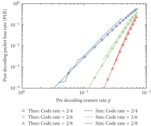
Figure 2: Packet loss rate for systematic codes with k = 2 but differentdmin.

where p represents the raw PLR. The PLR performance is

independent of the actual packet length; however the latter determines the percentage of overhead related to padding the

packets to the desired length determined bygmax. Also, since

the performance of the designed codes is characterized by the minimum distance, it is not necessary to compare it with the performance of other codes.

Figure 1shows the PLR performance for three codes with the same minimum distance of three and the same packet

size of 1000 bits but different code rates. The three codes

have the parameters (4, 2, 3), (7, 5, 3), and (14, 12, 3). The rates of these codes are 2/4, 5/7, and 12/14, respectively. We can observe that the performance improves as the code rate decreases because the codes can recover two packets in a

group ofncoded packets wheren=4, 7, and 14.

Figure 2shows the PLR performance for three codes with

different minimum distances and different rates. The three

codes have the parameters (4, 2, 3), (6, 2, 5), and (8, 2, 7). The

rates of these codes are 2/4, 2/6, and 2/8, while the minimum

distances are 3, 5, and 7, respectively. We can observe that the performance improves as the code rate decreases because they can recover 2, 4, and 6 packets, respectively. We can observe also that the theoretical PLR performances as given

by (17) agree with the simulation results.

6. Modified Erasure Designs

In this section, two modifications are introduced in order to lower the amount of zero padding needed. In the first modification, the shift elements are chosen and positioned

in the parity matrixPsuch that the determinant of the new

matrix U, replacingV, has a lower degree. A lower degree

determinant implies less zero padding for the packets and

hence a reduced overall overhead. The new parity matrixUis

such that all its submatrices are invertible. We show some of

that the new designed matrices and their submatrices are invertible by finding the inverses using simulations. Also,

the maximum degree determinant is calculated for U. A

comparison to the same size Vandermonde-based designs is shown.

6.1. Various Sizes Matrix Designs. The best design found that satisfy the invertibility condition using exhaustive search for

the 3×3 matrix is

The matrix in (18) is a nonVandermonde matrix. The

invertibility of this matrix and its submatrices is proven by using brute force simulations. This is done by finding all the

submatrices of (18) and calculating the determinants of these

submatrices. For this matrix, we found inverses for one 3×3

matrix, nine 2×2 submatrices, and nine 1×1 submatrices.

The number of submatrices that have inverses complies with

the maximum number in (10), meaning that the design is

invertible for any submatrix. This design has a maximum degree determinant of four compared to its corresponding Vandermonde matrix design which has a maximum degree determinant of five.

The two designs

⎡

are good candidates for the parity coefficient matrices of

sizes 4×4 and 5×5, respectively. These two matrices are

nonVandermonde matrices and invertible. The 4×4 design

has a maximum degree determinant of 11 compared to its corresponding Vandermonde matrix design, which has

a maximum degree determinant of 14. The 5 ×5 design

has a maximum degree determinant of 21 compared to its corresponding Vandermonde matrix design, which has a maximum degree determinant of 30.

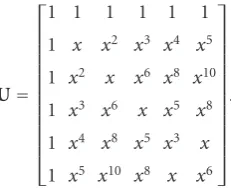
For the 6×6 matrix, the best design found is given by

U=

The matrix in (20) is also a nonVandermonde matrix.

For each square size matrix, Table 1 shows the number

of submatrices, the maximum degree determinant among

Table 1: The Maximum Degree Determinant in 6×6 Matrix Design.

Vandermonde nonVandermonde # of Submatrices

1×1 25 10 36

them, and a comparison with the corresponding same size Vandermonde design. The number of submatrices having

inverses complies with the maximum number in (10). This

design has a maximum degree determinant of 33 compared to its corresponding Vandermonde matrix design, which has a maximum degree determinant of 55.

Higher dimension matrices can also be designed and found in the same manner by generating the elements of the required size matrix and then testing the invertibility of each submatrix using brute force simulation.

The second modification that also will reduce the amount of zero padding is to zero pad with the maximum shift in the designed matrix, not with the maximum degree of the determinant. At the encoder side, each packet will be padded with the maximum shift in the matrix. Then at the receiver side, before starting decoding, the received packets are extra padded with zeros to make the total number of zero padding equal to the maximum degree determinant. This reduces the amount of overhead in the transmitted packets. This modification applies for any design (Vandermonde or nonVandermonde), and the advantages

benefit equally both modifications. For example, for a 6×6

Vandermonde matrix, 55 zeros are needed originally, while only 25 zeros are needed if we adopt the second modification, since the maximum shift in the Vandermonde matrix design

is 25. For a 6×6 nonVandermonde matrix, 33 zeros are

needed originally, while only 10 zeros are needed if we adopt the second modification, since the maximum shift in the

nonVandermonde matrix design in (20) is 10.

6.2. Simulation Results. This section shows post decoding

packet loss recovery performance, PLRpost, of the modified

nonVandermonde codes for a wide range of raw PLR in the network. For comparison purposes, the performance of the corresponding Vandermonde based designs are also plotted.

Figure 3 shows the PLR performance for five codes

with different minimum distances, but the same code rate

of 1/2 and the same packet size of 1000 bits. The five codes have the parameters (4, 2, 3), (8, 4, 5) Vandermonde-based, (8, 4, 5) nonVandermonde based (Modified), (12, 6, 7) Vandermonde-based, and (12, 6, 7) nonVandermonde based (Modified). The minimum distances are 3, 5, and 7,

respec-tively. By receiving any k packets, each code can recover

the remaining r = k packets. As the channel condition

that the performance improves as the minimum distance of the code increases. Also, we observe that the modified designs (nonVandermonde) and the original designs (Van-dermonde) have identical performances.

7. Error Correction Capability and Performance

In this section, the general error correction capability and the decoding process using the designed codes are presented. An error decoding technique capable of correcting a single erroneous packet irrespective of the number of errors in this packet is presented. We demonstrate the packet error rate (PER) reduction capability of these codes based on the proposed error decoding technique through analytical

calcu-lations and simulation results for different code parameters.

We assume here that there is no packet loss. Therefore,

at the receiver, all the coded packetsPare received. From the

received packets arranged row-wise in a matrixR, we have to

infer first which packet(s) is(are) in error, and then, within this(these) packet(s), where the error locations are and their values. For binary codes considered in this paper, the error values are not required, since by knowing their positions, one just flips them. There are many procedures that could correct

for errors by observingR. A typical way is to use syndrome

decoding which proceeds by finding the parity check matrix

H. The parity check matrix,H, ofGin (7) is then×rmatrix

whereVis the transpose ofV. Accordingly, the

multiplica-tion of the two partimultiplica-tioned matrices,HandGgives the zero

matrix.

Now assume that the n coded packets arranged in P

are transmitted and they are corrupted by errors. The received packets can be viewed as the coded packet corrupted (modulo-2 added) with packets having 1’s in the error locations. These packets are referred to as error packets and

are arranged row-wise in E, where the latter is a column

vector consisting of the elements Ei,i = 0,. . .,n−1. The

received packets arranged in the matrixRare given by

R=P+E=

whereRis a column vector consisting of the received packet

Ri(i=0,. . .,n−1). By pre-multiplying (22) byH, one gets

the packet syndrome denoted bySas follows:

S=H·R=H·E. (23)

If S=_/0, we have the indication that there were errors

during the transmission. It is observed that this syndrome

decoding technique in (23) depends only on the error

patterns,E, but not on the transmitted coded packets,P. The

syndrome decoding technique enables the code to correct for

tpacket(s) irrespective of the number of bits in error inside

the packet(s). A packet is considered in error if at least one bit of the packet is in error.

We show next how the syndrome decoding is utilized

to correct a single erroneous packet in a group of n

received packets. Extending the technique to correct for more erroneous packets needs further study and is beyond the scope of this paper.

For the MDS codes capable of correcting single erroneous

packet out of n packets, dmin = n−k+ 1 = 3; that is,

r=2 and thusn=k+ 2. Now we pre-multiply the resultant

syndrome equation in (23) by the matrix Q, which is the

column-wise reverse ofH[4]. We call the resultant matrix,

the error locator matrixW, which is given as follows:

W=Q·H·E, (24)

and (·)crrepresents column-reversed matrix. By substituting

(25) in (24), one gets (26):

where (·)rrrepresents row-reversed matrix. By carrying out

W=

are zeros. This means that if all the error packets are zeros

except one error packetEi, the only all-zero row inWwill

be the rowWi, wherei∈[0,n−1]. Also, we notice thatEi

corresponds to the last row in the error locator matrixW.

This is true except for the last oneEi=En−1=Ek+1, in which

case any row in the error locator matrix is the error packet. We would like to mention that the above technique needs more careful processing to handle the scenario that the error packet and a shifted version of it produce the same packet such as the all-ones error packet. Although the occurrence of such scenario is extremely small, especially for long packets, it can be handled by padding the packets resulting from the

syndrome equation with (r −1)·(k−1) zeros and then

discarding these zeros when finding the error packet. These zeros are not counted as an overhead since they are padded at the receiver side.

7.1. Error Correction Designs. In this section, we discuss some specific cases for the design of packet-level error correction codes proposed in this paper. First, we consider the (4, 2, 3) systematic code and present the decoding process without

using W, and then we demonstrate the benefits of error

locator matrix in this example. This code is capable of correcting one packet in error out of the received four packets. The generator and the parity check matrices are

G =

, respectively. At the receiver

side, the decoding process starts by applying the syndrome

decoding in (23) to get the following:

S=H·E=

From (28), if the error occurs in the first received packetR0,

the only packet that is not all-zero isE0 whileE1 = E2 =

E3=0. Therefore, the two packets comprising the syndrome

matrixS, in (28), are identical and are the error packet,E0,

itself. To correct the erroneous packetR0, one adds to it one

of the packets obtained from the syndrome calculation. If the

error occurs in the second received packet R1, the second

packet of the syndrome is a shifted version by one of the first packet in the syndrome. To correct the erroneous packet

R1, add it to the first packetE1 of the syndrome matrix. If

the error occurs in the third received packetR2, the second

packet of the syndrome is the all-zero packet, while the first

packet in the syndrome is the error packet E2. To correct

the erroneous packet R2, add to it the first packet of the

syndrome matrix. If the error occurs in the fourth received

packetR3, the second packet of the syndrome is the error

packet E3 while the first packet is the all-zero packet. To

correct the erroneous packetR3, add it to the second packet

of the syndrome matrix.

The above correction can be done more efficiently by

finding the error locator matrix W using (24). By

pre-multiplying the resultant syndrome equation in (28) byQ,

Wis found to be

The above error locator matrix reduces to the first, second,

third, or fourth column inTable 2when the packet in error

is the first, second, third, or fourth one, respectively. For example, if the packet in error is the fourth received packet

R3,E3 will be nonzero packet whileE0 = E1 = E2 = 0.

Therefore, based on (29),W reduces to the fourth column

in Table 2. This means that if we getW with the last row comprised of all-zeros, we decide that the erroneous packet is

the fourth one. In this case,E3can be taken either as the first,

second, or third packet in the fourth column ofW. When the

100 ₁₀−1 ₁₀−2

Pre decoding erasure ratep

10−4

Vandermonde: Code rate=4/8 Modified: Code rate=4/8 Vandermonde: Code rate=6/12 Modified: Code rate=6/12

Figure3: Packet loss rate for systematic codes with the same code rate of 1/2 but differentdmin.

before that the zero in the error locator matrix indicates the location of the packet in error and the error packet can be

taken as the last packet in the error locator matrix inTable 2.

The (5, 3, 3) systematic code is capable of correcting one packet in error out of the received five packets. By following

the procedure from (26), the error locator matrixWfor this

code is as follows:

W=Q·

The above error locator matrix reduces to the first, second,

third, fourth, or fifth column in Table 3 when the packet

in error is the first, second, third, fourth, or fifth one, respectively, in a block of 5 received packets. We notice as before that the zero in the error locator matrix indicates the location of the packet in error. Also, the error packet that should be added to correct the erroneous packet is the last row in the error locator matrix. This is true except when the

Table2: The error locator matrix,W, for a single packet in error for the (4, 2, 3) systematic code.

R0in error R1in error R2in error R3in error

Table3: The error locator matrix,W, for a single packet in error for the (5, 3, 3) systematic code.

R0in error R1in error R2in error R3in error R4in error

last received packet is in error, in which case any row in the error locator matrix is the error packet.

We discussed two codes (4, 2, 3) and (5, 3, 3) which are both single error correcting code like the (7, 4, 3) Hamming code. However, the rates of these three codes are 35/70, 42/70, and 40/70, respectively. The decoding process for the first

code is simple, but the code has a rate of 0.5. The decoding

process of the second code is a little bit more involved compared to the first one, but the code has a higher rate of

0.6. Higher rate single error correcting codes can be designed,

but the decoding complexity increases slightly as the code rate increases.

We presented an efficient decoding algorithm to correct

a single erroneous packet in a family of codes having a minimum distance of three. Therefore, this family is capable of correcting all bits in error within a single erroneous packet, irrespective of the size of the packet. The family has the

parameters (k+ 2,k, 3), wherek≥2. The rate of this family

is k/(k+ 2). This designed family has more flexible code

parameters when compared to the family of Hamming codes

having the parameters (2m_{−1, 2}m_{−m−1, 3), wherem≥3.}

The next Hamming code after the (7, 4, 3) is the (15, 11, 3)

which has a code rate of 11/15=0.733. A comparable code

performance in our design is when takingk=6 to construct

the code (8, 6, 3) having a code rate of 6/8=0.75. However,

the latter is less complex since it has a code length of 8, which is almost half of the Hamming code of length 15. As a result, the delay in constructing the encoder and decoder matrices is greatly reduced, especially as the code rate increases.

7.2. Simulation Results. This section shows postdecoding

packet error rate performance, PERpost, of the proposed

codes for a wide range of raw PER in the network.

100 ₁₀−1 ₁₀−2

Pre decoding error ratep

10−4

10−3

10−2

10−1

100

P

o

st

dec

o

ding

pac

ket

er

ro

r

rat

e

(P

E

R)

Theo: Code rate=2/4 Theo: Code rate=5/7 Theo: Code rate=12/14

Sim: Code rate=2/4 Sim: Code rate=5/7 Sim: Code rate=12/14

Figure4: Packet error rate for systematic codes withdmin=3.

decoding processes. The PER recovery simulation results are plotted using continuous unmarked lines. For comparison purposes, we also plot the theoretical curves using

continu-ous marked lines based on (17) but taking the summation

fromt+ 1 witht=1 instead ofe+ 1 andprepresenting here

the raw PER.

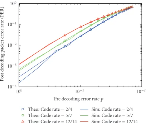
Figure 4shows the PER performance for three codes with

the same minimum distance of three but different code rates.

The three codes have the parameters (4, 2, 3), (7, 5, 3), and (14, 12, 3). The rates of these codes are 2/4, 5/7, and 12/14, respectively. We can observe that the performance improves as the code rate decreases because the codes can correct

for one packet in a group of n coded packets where n =

4, 7, and 14. Also, it can be noted that the theoretical PER performances agree with the simulation results.

8. Conclusion

We summarize now the advantages of working with the proposed code design for packet-level FEC in which the elements of the Vandermonde matrix are the shift operator. The code design is applicable to recover from lost packets up

ton−kout of thencoded packets, or correct one erroneous

packet out of thenreceived packets. This design is simple to

implement since all our arithmetic operations are done in the binary field using only simple shifts and modulo-2 additions. The only disadvantage is the overhead associated with the need to zero pad each packet with the maximum degree,

gmax, of the determinants among the set of all determinants

of square submatrices of the designed Vandermonde matrix. To reduce the overhead considerably, however, we proposed modified nonVandermonde matrix designs which were found by exhaustive search. We believe that finding such designs in more structured way is still a challenging problem especially as the matrix size increases. To even further reduce this overhead in both designs, we can only zero pad with the

maximum shift in the matrix which is much less thangmax.

The overhead reduces the efficiency of the design (overall

code rate) especially when designing for large code

param-eters. However, as the packets size increases, the efficiency

improves. Therefore, the design is applicable to packets of any size provided that they are not very small. For moderate code parameters, packets of few hundred bits (all network standards requires even more than this) are good enough

that will not affect the efficiency of the code very much.

For large code parameters, the efficiency can be improved by

increasing the packet size and/or by utilizing the mentioned ways of reducing the overhead.

For erasure recovery, we showed how to find the inverse of a matrix using a simple algorithm by exploiting the logarithmic operator of the elements of the Vandermonde matrix and converting the operations to simple modulo-2 additions. For error correction, we presented a syndrome decoding algorithm that corrects for a single erroneous packet using a specialized error locator matrix. The design is suitable for real-time applications and multicasting, where conventional ARQ protocols employing retransmission are inadequate, due to the introduction of delay and jitter. Also, the design can be exploited in cross-layer protocols design to recover from both erasures and errors simultaneously.

Acknowledgment

The authors acknowledge the support of King Fahd Univer-sity of Petroleum and Minerals (KFUPM).

References

[1] D. J. Costello, J. Hagenauer, H. Imai, and S. B. Wicker, “Applications of error-control coding,”IEEE Transactions on Information Theory, vol. 44, no. 6, pp. 2531–2560, 1998. [2] M. G. Luby, M. Mitzenmacher, M. A. Shokrollahi, and

D. A. Spielman, “Efficient erasure correcting codes,” IEEE Transactions on Information Theory, vol. 47, no. 2, pp. 569– 584, 2001.

[3] S. Karande and H. Radha, “Partial Reed Solomon codes for erasure channels,” in Proceedings of the IEEE Information Theory Workshop (ITW ’03), pp. 82–85, April 2003.

[4] A. Al-Shaikhi, Innovative designs and deplyments of erasure codes in communication systems, Ph.D. dissertation, Dalhousie University, Nova Scotia, Canada, 2007.

[5] R. L. Collins and J. S. Plank, “Assessing the performance of erasure codes in the wide-area,” in Proceedings of the International Conference on Dependable Systems and Networks (DSN ’05), pp. 182–187, Yokohama, Japan, June 2005. [6] S. Lin and D. J. Costello,Error Control Coding, Prentice-Hall,

Upper Saddle River, NJ, USA, 2004.

[7] S. S. Karande and H. Radha, “The utility of hybrid error-erasure LDPC (HEEL) codes for wireless multimedia,” in

Proceedings of the IEEE International Conference on Commu-nications (ICC ’05), vol. 2, pp. 1209–1213, Seoul, South Korea, May 2005.

[8] A. Al-Shaikhi, J. Ilow, and X. Liao, “An adaptive FEC-based packet loss recovery scheme using RZ turbo codes,” in

[9] A. A. Al-Shaikhi and J. Ilow, “Packet loss recovery codes based on Vandermonde matrices and shift operators,” inProceedings of the IEEE International Symposium on Information Theory (ISIT ’08), pp. 1058–1062, Toronto, Canada, July 2008. [10] F. J. Ayres, Schaum’s Outline of Theory and Problems of

Matrices, Schaum, New York, NY, USA, 1962.

[11] A. Ben-Israel and T. N. Greville,Generalized Inverses: Theory and Applications, Wiley Interscience, New York, NY, USA, 1977.

[12] D. S. Dummit and R. M. Foote,Abstract Algebra, Prentice-Hall, Englewood Cliffs, NJ, USA, 1998.

[13] J. Lacan and J. Fimes, “Systematic MDS erasure codes based on Vandermonde matrices,”IEEE Communications Letters, vol. 8, no. 9, pp. 570–572, 2004.

[14] J. Fimes, J. Lacan, et al., “Estimation of the number of singular square submatrices of Vandermonde matrices defined over a finite field,” Tech. Rep. RE-2003-01, ENSICA, January 2003. [15] F. MacWilliams and N. Sloane,The Theory of Error-Correcting

Codes, North Holland, Amsterdam, The Netherlands, 1978. [16] T. Muir,Treatise on the Theory of Determinants, Dover Phoenix