R E S E A R C H
Open Access
Neimark–Sacker bifurcation and stability
analysis of a discrete-time prey–predator
model with Allee effect in prey
Figen Kangalgil
1**Correspondence:
1Department of Mathematics,
Faculty of Science, Cumhuriyet University, Sivas, Turkey
Abstract
In this paper, the dynamical behaviors of a discrete-time prey–predator model with Allee effect on the prey population are investigated. The existence and topological classification of the fixed points of the model are analyzed. It is shown that the model can undergo a Neimark–Sacker bifurcation at the unique positive fixed point by choosingaas a bifurcation parameter. The conditions of the existence for
Neimark–Sacker bifurcation and the direction of bifurcation via bifurcation theory are presented. Also, some numerical simulations are presented to support of the analytical finding. Then bifurcation diagrams and phase portraits of the model are given.
MSC: 39A28; 39A30; 92B05
Keywords: Allee effect; Prey–predator model; Stability
1 Introduction
The predator–prey models have a theoretical and practical significance. So many authors have studied the dynamics of these models. The Lotka–Volterra model is the first and the simplest model of predator–prey interactions. The model was developed independently by Lotka [1] and Volterra [2]. The Lotka–Volterra model assumes that the prey consump-tion rate by a predator is directly proporconsump-tional to the prey abundance. This means that predator feeding is limited only by the amount of prey in the environment. While this may be realistic at low prey densities, it is certainly an unrealistic assumption at high prey densities where predators are limited, for example, by time and digestive constraints. So a number of changes in the model have been presented by researchers to include Holling type functional responses and density-dependent prey growth. Another way of modifica-tion of the Lotka–Volterra model can be considered by introducing the Allee effect. It is well known that the introduction of the Allee effect into the system is more realistic in modeling the prey–predator interaction.
The Allee effect is a crucial phenomenon that has drawn considerable attention from both theoretical and applied ecologists [3–9]. The Allee effect was first described by Allee in 1931 [10]. It describes a positive correlation between any measure of species fitness and population numbers. The main causes of the Allee effect are the difficulty in finding mates, inbreeding depression, social dysfunction at small population sizes, predator avoidance
and food exploitation [11–14]. Empirical evidence of the Allee effect has been observed in many natural species, for example, plants [15], insects [16], marine invertebrates [17], birds and mammals [18]. Recent studies have shown that the Allee effect has important dy-namical effects on the stability analysis of population models. The system with Allee effect shows either destabilization [11] or stabilization [19]. The local stability of a positive fixed point may be changed from stable to unstable or vice versa. In prey–predator systems, Allee effect may change the dynamics of the system in unexpected ways and induce com-plex dynamics. So, many authors have investigated the stabilizing or destabilizing effects on the predator–prey models with the Allee effect. But the bifurcation analysis of these systems with the Allee effect has been rarely performed. So, in this paper, a predator–prey system on which is imposed an Allee effect is considered.
In [20], the author has considered the following discrete-time predator–prey model which was proposed by Smith et al. [21]:
Xt+1=αXt(1 –Xt) –XtYt,
Yt+1= 1
βXtYt,
(1)
whereXtandYtdenotes the numbers of prey and predator respectively. The parametersα, βare positive real numbers. They have studied stability and Neimark–Sacker bifurcation of a discrete-time predator–prey model. The analysis of bifurcations has already received much attention during the last few years [20,22–29]. Bifurcation and stability analysis are examined in detail in [20,22–24,30–41].
In this paper, modification of the model (1) is considered by introducing the Allee effect for the prey population as follows:
Xt+1=aXt(1 –Xt) –XtYt
Xt
m+Xt
,
Yt+1= 1
βXtYt,
(2)
where X
m+Xis term for the Allee effect.m> 0 can be defined as Allee effect constant [11–
13].αandβare the growth rates of the prey and predator, respectively.
The aim of this paper is to investigate the dynamics of a modified a discrete-time predator–prey model with Allee effect on prey population by using bifurcation theory. The rest of the paper is organized as follows: In Sect.2, the existence conditions and sta-bility of the fixed points are discussed. In Sect. 3, choosingaparameter as bifurcation parameter, Neimark–Sacker bifurcation analysis is studied. Furthermore, by using normal form theory direction of Neimark–Sacker bifurcation is obtained. Finally, these theoretical results are supported by some numerical simulations.
2 The fixed points: existence and stability
In this section, we will study the existence of the fixed points of the discrete system with Allee effect and analyze the stability of these fixed points. To find the fixed points of the system (2), we can write
in the model (2)
X∗=aX∗1 –X∗–X∗Y∗
X∗ m+X∗
,
Y∗=1
βX ∗Y∗.
(4)
It is clear that the fixed points of the model (2) satisfy Eq. (4).
Lemma 1
(i) The system(2)always has an axial fixed pointE1= (0, 0). (ii) The system(2)has an axial fixed pointE2= (a–1a , 0)ifa> 1.
(iii) The system(2)has a unique positive fixed pointE∗= (β,(β+m)(aβ(1–β)–1))ifa>
1 1–β andβ< 1.
In order to analyze the stability of the fixed points of the model (2), we give Definition1
and Lemma2as follows:
Definition 1 A fixed point (N,P) is called
(i) sink if|λ1|< 1and|λ2|< 1, and it is locally asymptotically stable, (ii) source if|λ1|> 1and|λ2|> 1, and it is locally unstable,
(iii) saddle if|λ1|< 1and|λ2|> 1or (|λ1|> 1and|λ2|< 1), (iv) non-hyperbolic if either|λ1|= 1or|λ2|= 1.
To investigate the stability of the one nontrivial fixed point of the system (2), we give Lemma2.
Lemma 2 Assume F(λ) =λ2+Bλ+C,where B and C are two real constants and let F(1) > 0. Supposeλ1andλ2are two roots of F(λ) = 0.Then the following statements hold.
(i) |λ1|< 1and|λ2|< 1if and only ifF(–1) > 0andC< 1; (ii) |λ1|> 1and|λ2|> 1if and only ifF(–1) > 0andC> 1;
(iii) |λ1|< 1and|λ2|> 1,or|λ1|> 1and|λ2|< 1,if and only ifF(–1) < 0;
(iv) λ1andλ2are a pair of conjugate complex roots and|λ1|=|λ2|= 1if and only if B2– 4C< 0andC= 1;
(v) λ1= –1and|λ2| = 1if and only ifF(–1) = 0andB= 0, 2.
Now we will discuss the topological classification of the fixed points of the model (2) and we will apply Lemma2to prove the following lemmas.
The Jacobian matrix of the planar map in (2) evaluated at any point (x,y) is given by
J(x,y) =
a(1 – 2x) –x2+xym +(x+x2my)2 – x 2 x+m y
β
x β
and we have
Lemma 3 For the fixed point E1(0, 0),following topological classification holds: (i.1) E1(0, 0)is a sink ifa< 1.
The characteristic equation of matrixJ(E∗) can be written as follows:
F(λ) =λ2– (a11+a22)λ+ (a11a22–a12a21), (6)
system(2)the following holds true.
(iii1) E∗is sink fixed point if the following condition holds:
1
(iii2) E∗is source fixed point if the following condition holds:
1
1 – 2β–m<a<
3β+ 5m 3β2+βm+m–β,
(iii3) E∗is saddle fixed point if the following condition holds:
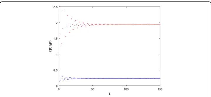
Figure 1A stable fixed point for the system (2) fora= 2.5,m= 0.25,β= 0.23 and initial condition (x0,y0) = (0.15, 2.5)
(iii4) non-hyperbolic fixed point if the following conditions hold:
a= 3β+ 5m
3β2+βm+m–β and m= 4 5–
9 5β,
(iii5) the roots of Eq. (7)are complex with modules one if and only if
a= 1
1 – 2β–m and m< 4 5–
9 5β.
Example 1 For the parameter values a= 2.5, m= 0.25, β = 0.23 and initial condi-tion (x0,y0) = (0.15, 2.5), the positive fixed point of the model (2) is obtained: (x∗,y∗) = (0.23, 1.930434783). Figure1is shown that the fixed point (x∗,y∗) of the model (2) is lo-cal asymptotilo-cally stable where blue and red graphs representx(t) and y(t) population, respectively.
3 Bifurcation analysis
3.1 Neimark–Sacker bifurcation at the pointE∗
In this section we investigate the conditions for existence of the Neimark–Sacker bifurca-tion for unique positive fixed pointE∗= (β,(β+m)(aβ(1–β)–1)) of the model (2). Also, direction of Neimark–Sacker bifurcation is evaluated. We will takeaas bifurcation parameter.
Let us consider the term ofΩNSBE∗ as follows:
ΩNSBE∗=
(a,β,m)∈R3:a= 1
1 – 2β–m,m< 4 5–
9
5βandβ< 1
2 . (9)
When the parameters change in small neighborhood ofΩNSBE∗, two eigenvalues ofJ(E
∗)
are complex having magnitude one and Neimark–Sacker bifurcation can go out from the fixed pointE∗. The eigenvalues of Eq. (2) under these conditions are given by
λ,λ=(–3m+ 5β– 2)±i √
β+m√4 – 5m– 9β
It is easy to see that
|λ|=|λ|= 1. (11)
From the transversality condition, we get
d|λi(a)|
NSBE∗) and transposed matrix JT(Ω
NSBE∗) corresponding toλandλ, respectively. We have
q∼
To achieve the normalizationp,q= 1, where,means the standard scalar product in C2, we can take the normalized vectors as
q=
where
The system (19) can be expressed as
are symmetric multilinear vector func-tions ofx,y,u∈R2. These functions are defined as follows:
The system (19) can be transformed for all sufficiently small|a|into the form
whereλ(a) = (1 +ϕ(a))eiarctan(a) withϕ(a
NS) = 0 andg(z,z,a) is smooth complex-valued
function. After taking the Taylor expression ofgwith respect to (z,z), we obtain
g(z,z,a) =
By symmetric multilinear vector functions, the Taylor coefficientsgklcan be expressed
by the formulas
The coefficientβ2(aNS), which determines the direction of the appearance of the invariant
curve in a generic system exhibiting the Neimark–Sacker bifurcation, can be calculated via
We state the following theorem on the Neimark–Sacker bifurcation.
Theorem 1 Suppose that E∗is positive fixed point of the model(2).If(13)holds, 1 – 2β– m= 0,β2(aNS)= 0and the parameter a changes its value in small vicinity ofΩNSBE∗,then the model(2)passes through a Neimark–Sacker bifurcation at only fixed point E∗.
More-over,ifβ2(aNS) < 0 (resp.,β2(aNS) > 0),then the Neimark–Sacker bifurcation of model(2)at
a=aNSis supercritical(resp.,subcritical)and there exists a unique closed invariant curve
bifurcation from E∗for a=aNS,which is attracting(resp.,repelling).
4 Numerical simulations
In this section, our aim is to present numerical simulations to validate the above the-oretical results, especially the bifurcation diagrams and phase portraits for system (2) around fixed point E∗. We will choosea as the bifurcation parameter. The Neimark–
Sacker bifurcation point asaNS= 3.448275862 is obtained. By taking the parameters
val-uesaNS= 3.448275862,m= 0.25 andβ= 0.23, the positive fixed point of the model (2) is
evaluated asE∗= (0.23, 3.454150957).
Using the above the parameters, we get the jacobian matrix as follows:
The eigenvalues are evaluated as follows:
λ1,2= 0.1724582115±0.9850322777i.
Letq,p∈C2be complex eigenvectors corresponding toλ
1,2, respectively.
q∼(–0.06558990232 – 0.05510315377i,i)T
and
p∼(8.937911026 – 7.508885793i, –i)T.
To obtain the normalizationp,q= 1, we can take normalized vectors as
q= (–0.06558990232 – 0.05510315377i,i)T
and
p=–7.623124629 + 0.2149349453.10–8i, –0.4200582087 + 0.5000000001iT.
Because of computing the coefficients of normal form, we transform the point (0, 0) to the fixed pointE∗by a change of variables,
X=x– 0.23,
Y=y– 3.454150957.
So, we can compute the coefficients of the normal of the system by using Eq. (24) as follows:
g20(δ) = –2.007675632 – 0.1335717640i,
g11(δ) = 2.430928813 + 0.2395789296i,
g02(δ) = 1.186267438 – 2.549712245i,
g21(δ) = 0.1518172527 + 0.1907737437i.
From (25), the critical part is obtained: β2(aNS) = –8.214126411 < 0. Therefore, the
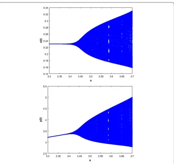
Neimark–Sacker bifurcation is supercritical and it shows the correctness of Theorem1. The bifurcation diagram and the phase portrait of the system (2) is shown in Figs.2and3. The bifurcation diagrams shown in Fig.2show that the stability ofE∗holds fora< 3.4482
and loses its stability ata= 3.4482 and an attracting invariant curve appears ifa> 3.4482. The phase portraits of bifurcation diagrams in Fig.2for different values ofaare dis-played in Fig.3, which clearly depicts the process of how a smooth invariant circle bifur-cates from the stable fixed pointE∗= (0.23, 3.454150957). Whenaexceeds 3.448275862
there appears a circular curve enclosing the fixed pointE∗, and its radius becomes larger
Figure 2Bifurcation diagram for the system (2) for values ofm= 0.25,β= 0.23,a= 3.3 : 0.0001 : 3.4 and initial value (x0,y0) = (0.2, 3.4)
Figure 3Phase portraits of the system (2) for different values ofa
5 Discussions
given. By bifurcation theory [39–41] we showed that the system (2) undergoes a Neimark– Sacker bifurcation at unique coexistence fixed point if a varies around the setΩNSBE∗. The parametric conditions for existence and direction of Neimark–Sacker bifurcation in posi-tive fixed pointE∗were given. Also, we verified the theoretical results by presenting some
numerical simulations and phase portrait diagrams using MATLAB. We displayed that when the bifurcation parameterapasses a critical bifurcation value, stability of the coex-istence equilibrium point of the model (2) changes from stable to unstable and Neimark– Sacker bifurcation occurs at this critical value. Therefore, we can say that the parametera has a strong effect on the stability of the system so as control two populations.
Acknowledgements
The authors would like to thank the referee and the editor for their valuable comments, which led to improvement of this work.
Funding
Not applicable.
Availability of data and materials
Not applicable.
Competing interests
The authors declare that they have no competing interests.
Authors’ contributions
All authors read and approved the final manuscript.
Publisher’s Note
Springer Nature remains neutral with regard to jurisdictional claims in published maps and institutional affiliations.
Received: 30 March 2018 Accepted: 22 February 2019
References
1. Lotka, A.J.: Elements of Mathematical Biology. Williams & Wilkins, Baltimore (1925)
2. Volterra, V.: Variazioni e fluttuazioni del numero di’ individui in specie animali conviventi. Mem. R. Accad. Naz. Dei Lincei, Ser. VI2, 31–113 (1926)
3. Birkhead, T.R.: The effect of habitat and density on breeding success in the common guillemot. J. Anim. Ecol.46, 751–764 (1977)
4. Dennis, B.: Allee effect: population growth, critical density, and the chance of extinction. Nat. Resour. Model.3, 481–538 (1989)
5. McCarthy, M.A., Lindenmayer, D.B., Dreschler, M.: Extinction debts and risks faced by abundant species. Conserv. Biol.
11, 221–226 (1997)
6. Amarasekare, P.: Interactions between local dynamics and dispersal: insights from single species models. Theor. Popul. Biol.53, 44–59 (1998)
7. Drake, J.M.: Allee effects and the risk of biological invasion. Risk Anal.24, 795–802 (2004)
8. Shi, J., Shivaji, R.: Persistence in reaction diffusion models with weak Allee effect. J. Math. Biol.52, 807–829 (2006) 9. Taylor, C.M., Hastings, A.: Allee effects in biological invasions. Ecol. Lett.8, 895–908 (2005)
10. Allee, W.C.: Animal Aggretions: A Study in General Sociology. University of Chicago Press, Chicago (1931) 11. Zhou, S., Liu, Y., Wang, G.: The stability of predator–prey systems subject to the Allee effects. Theor. Popul. Biol.67,
23–31 (2005)
12. Kangalgil, F., Ak Gümü¸s, Ö.: Allee effect and stability in a discrete-time host-parasitoid model. J. Adv. Res. Appl. Math.
7, 1–6 (2016)
13. Kangalgil, F., Ak Gümü¸s, Ö.: Allee effect in a new population model and stability analysis. Gen. Math. Notes (2016) 14. Duman, O., Merdan, H.: Stability analysis of continuous population model involving predation and Allee effect. Chaos
Solitons Fractals41, 1218–1222 (2009)
15. Groom, M.J.: Allee effects limit population viability of an annual plant. Am. Nat.151, 487–496 (1998)
16. Kuussaari, M., Saccheri, I., Camara, M., Hanski, I.: Allee effect and population dynamics in the glanville fritillary butterfly. Oikos82, 384–392 (1998)
17. Stoner, A.W., Ray-Culp, M.: Evidence for Allee effects in an over-harvested marine gastropod: density-dependent mating and egg production. Mar. Ecol. Prog. Ser.202, 297–302 (2000)
18. Courchamp, F., Grenfell, B.T., Clutton-Brock, T.H.: Impact of natural enemies on obligately cooperative breeders. Oikos
91, 311–322 (2000)
19. Scheuring, I.: Allee effect increases the dynamical stability of populations. J. Theor. Biol.199, 407–414 (1999) 20. Khan, A.Q.: Neimark–Sacker bifurcation of a two-dimensional discrete-time predator–prey model. SpringerPlus5, 126
(2016)
22. Kartal, S.: Multiple bifurcations in an early brain tumor model with piecewise constant arguments. Int. J. Biomath.
11(4), 1850055 (2018)
23. Kartal, S., Gurcan, F.: Global behaviour of a predator–prey like model with piecewise constant arguments. J. Biol. Dyn.
9(1), 157–171 (2015)
24. Elabbasy, E.M., Elsadany, A.A., Zhang, Y.: Bifurcation analysis and chaos in a discrete reduced Lorenz system. Appl. Math. Comput.228, 184–194 (2014)
25. Zhang, J., Deng, T., Chu, Y., Qin, S., Du, W., Luo, H.: Stability and bifurcation analysis of a discrete predator–prey model with Holling type III functional response. J. Nonlinear Sci. Appl.9, 6228–6243 (2016)
26. Liu, X., Xiao, D.: Complex dynamics behaviors of a discrete-time predator–prey system. Chaos Solitons Fractals32, 80–94 (2007)
27. Rana, S.M., Kulsum, U.: Bifurcation analysis and chaos control in a discrete-time predator–prey system of Leslie type with simplified Holling type IV functional response. Discrete Dyn. Nat. Soc.2017, Article ID 9705985 (2017) 28. Hu, Z., Teng, Z., Zhang, L.: Stability and bifurcation analysis of a discrete predator–prey model with nonmonotonic
functional response. Nonlinear Anal., Real World Appl.12, 2356–2377 (2011)
29. Du, W., Zhang, J., Qin, S., Yu, J.: Bifurcation analysis in a discrete SIR epidemic model with the saturated contact rate and vertical transmission. J. Nonlinear Sci. Appl.9, 4976–4989 (2016)
30. Din, Q.: Neimark–Sacker bifurcation and chaos control in Hassel–Varley model. J. Differ. Equ. Appl.23(4), 741–762 (2016)
31. Din, Q.: Complexity and choas control in a discrete-time prey–predator model. Commun. Nonlinear Sci. Numer. Simul.49, 113–134 (2017)
32. Din, Q.: Bifurcation analysis and chaos control in a host–parasitoid model. Math. Methods Appl. Sci.40, 5391–5406 (2017)
33. Din, Q.: A novel chaos control strategy for discrete-time brusselator models. J. Math. Chem. (2018).
https://doi.org/10.1007/s10910-018-0931-4
34. Din, Q.: Stability, bifurcation analysis and chaos control for a predator–prey system. J. Vib. Control (2018).
https://doi.org/10.1177/1077546318790871
35. Din, Q.: Bifurcation analysis and chaos control in a second-order rational difference equation. Int. J. Nonlinear Sci. Numer. Simul.19(1), 53–68 (2018)
36. Din, Q.: Bifurcation analysis and chaos control in discrete-time glycolysis models. J. Math. Chem.56(3), 904–931 (2018)
37. Din, Q., Hussain, M.: Controlling chaos and Neimark–Sacker bifurcation in a host-parasitoid model. Asian J. Control
21(4), 1–14 (2019)
38. Din, Q.: Controlling chaos in a discrete-time prey–predator model with Allee effects. Int. J. Dyn. Control
https://doi.org/10.1007/s40435-017-0347-1
39. Kuznetsov, Y.A.: Elements of Applied Bifurcation Theory, 2nd edn. Springer, New York (1998)