R E S E A R C H
Open Access
Throughput analysis of buffer-constrained
wireless systems in the finite blocklength
regime
M Cenk Gursoy
Abstract
In this paper, a single point-to-point wireless link operating under queueing constraints in the form of limitations on the buffer violation probabilities is considered. The achievable throughput under such constraints is captured by the effective capacity formulation. It is assumed that finite blocklength codes are employed for transmission. Under this assumption, a recent result on the channel coding rate in the finite blocklength regime is incorporated into the analysis, and the throughput achieved with such codes in the presence of queueing constraints and decoding errors is identified. The performance of different transmission strategies (e.g., variable-rate, variable-power, and fixed-rate transmissions) is studied. Interactions and tradeoffs between the throughput, queueing constraints, coding blocklength, decoding error probabilities, and signal-to-noise ratio are investigated, and several conclusions with important practical implications are drawn.
Keywords: Buffer violation probability; Coding rate; Decoding error probability; Effective capacity; Fading channels; Finite blocklength regime; Quality of service constraints; Variable-rate/variable-power/fixed-rate transmissions
1 Introduction
Providing quality of service (QoS) guarantees in the form of limitations on the queueing delays or buffer violation probabilities is essential in many delay-sensitive wireless systems, e.g., voice over IP (VoIP), and wireless interactive and streaming video applications. Due to the importance of such QoS considerations, it is of significant interest to conduct an analysis and provide predictions for the performance levels of practical systems. In [1], effective capacity is proposed as a metric that can be employed to measure the performance in the presence of statisti-cal QoS limitations. Effective capacity formulation uses the large deviations theory and incorporates the statis-tical QoS constraints by capturing the rate of decay of the buffer occupancy probability for large queue lengths. Hence, effective capacity can be regarded as the maximum throughput of a system operating under limitations on the buffer violation probability.
Correspondence: [email protected]
Department of Electrical Engineering and Computer Science, Syracuse University, Syracuse, NY 13244, USA
Recently, there has been much interest in the analysis of the effective capacity of fading channels (see, e.g., [2-9]) in order to identify the performance of wireless systems operating under statistical queueing constraints. How-ever, in almost all prior studies, the service rates of the queueing model (or equivalently the instantaneous trans-mission rates over the wireless channel) are assumed to be equal to the instantaneous capacity values, although chan-nel coding is performed using a finite block of symbols. Moreover, transmissions are assumed to be reliable with no decoding errors. However, it is important to note that error-free communication at the rate of channel capac-ity is generally attained as the codeword length increases without bound. Therefore, when finite blocklength codes are employed, transmission is necessarily performed in the presence of decoding errors and possibly at rates less than the channel capacity in order to have high reliability or equivalently low error probability.
In [10] and [11], Negi and Goel addressed these con-siderations. They studied queueing and coding jointly and took explicitly into account decoding errors by consider-ing the random codconsider-ing exponents of error probabilities for rates less than the instantaneous channel capacity. For
instance, in [10], they analyzed the maximization of the joint exponent of the decoding error and delay violation probability through the appropriate choice of the trans-mission rate for a given delay bound and constant arrival rate.
In this paper, we also depart from the idealistic assump-tions of communicating arbitrarily reliably at channel capacity but follow an approach different from that of [10] and [11]. We consider channel coding rates achievable with finite blocklength codes and incorporate the decod-ing error probabilities and possible retransmission scenar-ios into the effective capacity formulation. This analysis is facilitated mainly by the recent results of Polyanskiy et al. [12], where the authors identified an approximate maximal achievable rate expression for a given error prob-ability in the finite blocklength regime. This expression can be regarded as a second-order asymptotic approx-imation of the channel coding rate at large but finite blocklength values. We note that [13] and [14] also stud-ied channel coding and achievable error probabilities at finite blocklengths by analyzing the mutual information density and its statistics. In [14], an outage analysis is performed by using the distribution of the mutual infor-mation density. In [15], a similar outage formulation is used to determine the optimal physical-layer reliability and to identify the maximum Automatic Repeat reQuest (ARQ) throughput. On the other hand, neither of the above-mentioned papers have investigated the through-put in the finite blocklength regime when the systems operate under buffer constraints.
Our contributions in this paper can be summarized as follows. We determine the throughput achieved by dif-ferent transmission strategies in the finite blocklength regime under constraints on the buffer violation probabil-ity. Initially, we consider a scenario in which the transmis-sion rate is varied with the fading realizations while the error probability is kept fixed. The optimal error probabil-ity that maximizes the throughput is shown to be unique. We analyze the impact of the power adaptations. Then, we investigate the case in which the transmission rate is fixed and error probability varies over different trans-mission blocks. Through numerical results, we analyze the interactions between the throughput, queueing con-straints, error probabilities, blocklength, signal-to-noise ratio, and different transmission strategies.
The remainder of the paper is organized as fol-lows. Section 2 describes the fading channel model. In Section 3, we provide preliminaries on the effective capac-ity as a measure of the throughput under statistical QoS constraints. In Section 4, we provide our results on the effective throughput in the finite blocklength regime when the transmitter sends the data at a variable rate with fixed power. In Section 5, we investigate the throughput in sce-narios in which power control is employed, or data is
transmitted at fixed rate, or independent messages are sent over two parallel channels. We conclude in Section 6. Several proofs are relegated to the Appendix.
2 Channel model
We consider a frequency-flat channel model and assume that the fading coefficients stay fixed for a block of m
symbols and then change independently for the follow-ing block. Under this block-fadfollow-ing assumption, the chan-nel input-output relation in one coherence block can be expressed as
y=hx+n (1)
wherexandyare them-dimensional, complex, channel input and output vectors, respectively. The input is sub-ject to an average power constraint, i.e.,E{x2} ≤ mP.
his the complex-valued fading coefficient with finite sec-ond moment, i.e., E{|h|2} < ∞. We assume that both
the receiver and transmitter have perfect channel side information (CSI) and hence perfectly know the instanta-neous realizations of the fading coefficients. However, the assumption of perfect CSI at the transmitter is relaxed in Section 5.2. Finally,nrepresents the Gaussian noise vector whose components are independent and identically dis-tributed (i.i.d.), complex, circularly symmetric, Gaussian random variables with mean zero and variance N0, i.e., n ∼ CN(0,N0Im), whereIm denotes them×midentity
matrix. We define the transmitted signal-to-noise ratio as
SNR= E{x
2}
E{n2} =
mP mN0 =
P N0
. (2)
Note that the received instantaneous signal-to-noise ratio for a given fading coefficienthis|h|2SNR.
3 Throughput under statistical queueing constraints
In [1], Wu and Negi defined the effective capacity as the maximumconstantarrival rate that a given service pro-cess can support in order to guarantee a statistical QoS requirement specified by the QoS exponent θa. If we defineQas the stationary queue length, thenθis the decay rate of the tail of the distribution of the queue lengthQ:
lim
q→∞
logP(Q≥q)
q = −θ. (3)
Therefore, for largeqmax, we have the following
approx-imation for the buffer violation probability:
P(Q≥qmax)≈e−θqmax.
Hence, while largerθ corresponds to more strict QoS constraints, smallerθimplies looser QoS guarantees. Sim-ilarly, ifDdenotes the steady state delay experienced in the buffer, thenP(D ≥ dmax) ≈ e−θ δdmax for largedmax,
[4]. Therefore, effective capacity formulation provides the maximum constant arrival rates that can be supported by the time-varying wireless channel under the queue length constraintP(Q ≥ qmax) ≤ e−θqmax for largeqmaxor the
delay constraintP(D≥ dmax) ≤ e−θ δdmax for largedmax.
Since the average arrival rate is equal to the average depar-ture rate when the queue is in steady state [16], effective capacity can also be seen as the maximum throughput in the presence of such constraints.
The effective capacity is given by ([1,17,18])
RE= −t→∞lim
stationary and ergodic stochastic service process. We would like to note that in the remainder of the paper, we will refer toREas the effective rate rather than the effective
capacity sinceREin our setup is the throughput when the
service rates are equal to the approximate channel coding rates in the finite blocklength regime.
4 Effective throughput with finite blocklength codes
4.1 Throughput in fading channels under QoS constraints In [12], the authors have studied the channel coding rate in the finite blocklength regime. For general classes of chan-nels, they have obtained new achievability and converse bounds on the coding rate for a given finite blocklength and error probability. In particular, for the real, additive white Gaussian noise (AWGN) channel, the transmission rate (in bits permchannel uses) with error probability 0< <1, signal-to-noise ratio (SNR), and coding blocklength
mis shown to have the following asymptotic expression ([12], Theorem 54): function. Denoting the rate in bits per channel use byr¯, we can write
where the approximation is accurate for sufficiently large
m. Note that the above results are for the AWGN channel with real input and real output.
In this paper, we consider a fading Gaussian chan-nel model with complex-valued input and output, and assume that channel coding is performed in each coher-ence interval of m symbols, during which the fading stays fixed. Under these assumptions, coding over a fad-ing Gaussian channel can be seen as codfad-ing over a real Gaussian channel (with a certain channel gain) using a coding blocklength of 2m. The following arguments pro-vide a detailed description of this approach. Knowing the channel fading coefficienth, the receiver can multiply the received signal withe−jθh, whereθ
inary components, respectively, of the output vector y˜, input vectorx, and noise vectorn˜. It can be easily veri-fied thatn˜ =ne−jθhhas the same statistics asnand hence
˜
n∼ CN(0,N0Im). Now, the above channel input-output
relation can also be written as
wherey˜r y˜idenotes the vector formed by concatenating
˜
yr andy˜i. Since the real and imaginary components are m-dimensional vectors, the above channel model is a real Gaussian channel with 2mdimensional input and output and with channel gain|h|. Note that the real and imagi-nary noise componentsn˜randn˜iare independent due to
the assumption of the circular symmetry of the additive complex Gaussian noise. For this channel, the coding rate (in bits permchannel uses) in theithblock achieved with block error probabilityis
ri=mlog2 1+SNR|hi|2−
where hi denotes the fading coefficient in theith block.
Note that the expression in (10) is obtained from that in (5) by replacingmwith 2m, and the signal-to-noise ratio with SNR|hi|2 = NP
0|hi|
2, which is the received
signal-to-noise ratio in theithblock. Now, the normalized rate in bits per channel use is approximately
for large enoughmfor whichO(log 2m m)is negligible. Hence-forth, we assume that the instantaneous transmission rate in each coherence block of the fading channel is given by the expression in (11). Since the block error rate is, this rate is attained with probability 1− . We assume that the receiver reliably detects the errors, employs a simple ARQ mechanism, and sends a negative acknowledgement requesting the retransmission of the message in case of an erroneous reception. Therefore, the data rate is effec-tively zero when error occurs. Under this assumption, the service rate (in bits permchannel uses) in each block is
Ri=
0 with prob.
mr¯i with prob.(1−) . (12)
With the above service rate characterization, we can express the effective rate (in bits per channel use) at a given SNR, error probability, blocklengthm, and QoS exponentθas
RE(θ )= − 1
mθlogeE|h|2
+(1−)e−θm¯r bits/channel use, (13)
where r¯ is given in (11), and the expectation is with respect to|h|2. The effective rate expression in (13) is eas-ily derived from (4) by noting that the service rate{Ri}is
an i.i.d. process due to the facts that the fading process is i.i.d. in different blocks, and the noise is an i.i.d. process leading to the independence of error events in different blocks.
Note that the effective rate is a function of the QoS exponentθ, blocklengthm, SNR, and error probability. Since we assume that coding is performed in each coher-ence interval, the blocklength m is determined by the statistics of the fading process. The value ofθ is dictated by the application requirements, and SNR depends on the power budget. Given the values of these parameters, the remaining parametercan be optimized to maximize the throughput.
Proposition 1.Assume that the values of m,θ >0, and SNR>0are fixed. Then, the function
()=E|h|2
+(1−)e−θm¯r (14)
is strictly convex in, and therefore, the optimal value of that minimizes this function or equivalently maximizes the effective rate in (13) is unique. Moreover, the effective rate REin (13) is a quasiconcave function of.
Proof. See Appendix 1.
Remark 1. Note that the strict convexity result indi-cates that the optimal error probability∗ is unique and can be easily found using standard convex optimization
methods. The analysis and the resulting∗provide guide-lines on the design of the channel codes and what their strength and protection level should be. Note that large
implies that the transmitter attempts to transmit the data at a high rate but at the risk of more frequent errors and hence retransmissions. On the other hand, if is small, the reliability of the transmissions is high but the instantaneous transmission rate is low. In either of these extreme regimes, the resulting throughput is low, which is not favorable in a buffer/delay limited system. The above result shows that a balance is struck at a unique value of the error probability, and this point can be identified with-out much difficulty for given buffer constraints specified byθ. Indeed, as will be seen in the numerical results,∗is not vanishingly small, indicating that some relatively small but nonzero error probability and hence some retrans-missions are allowed to improve the throughput of the system.
The above result is shown for the case in whichθ >0. If there are no QoS constraints and henceθ =0, then the effective rate becomes
RE(0)= lim
θ→0RE(θ )=(1−)E|h|2{¯r}, (15)
where r¯ is given in (11). Note thatRE(0) is the average
transmission rate averaged over the fading states. Below, we show thatRE(0)is a strictly concave function of.
Proposition 2.Assume that the values of m and SNR>
0are fixed. Then, the function
RE(0)=(1−)E|h|2{¯r} (16)
is strictly concave in, and therefore the optimal value of that maximizes this effective rate is unique.
Proof. See Appendix 2.
4.2 Numerical results
Next, we provide numerical examples to illustrate the results. Although the preceding analysis is applicable to any fading distribution with finite power, we consider a Rayleigh fading channel in the numerical analysis and assume that the fading powerz= |h|2is exponentially dis-tributed with unit mean (i.e., has the probability density functionfz(z)=e−z).
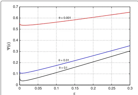
In Figure 1, we plot () = E|h|2
+(1−)e−θm¯r
0 0.05 0.1 0.15 0.2 0.25 0.3 0
0.1 0.2 0.3 0.4 0.5 0.6 0.7
ε
Ψ
(
ε
)
θ = 0.01
θ = 0.1
θ = 0.001
Figure 1The function()vs. the error probabilityin the Rayleigh fading channel.SNR=0 dB and the blocklength is
m=1, 000.
to ∗ = 0.0127, 0.0061, 0.0084 for θ = 0.001, 0.01, 0.1, respectively. It is also interesting to see that the opti-mal error probabilities are not vanishingly sopti-mall and are around 0.01.
In Figure 2, we plot the effective rate in (13) as a function of the error probability . The other param-eters are the same as in Figure 1. Notice that we have also included in this figure the throughput curve for the case in which θ =0. Note that if θ =0, the system does not have any queueing constraints. In Proposition 2, we have shown that RE(0) is a strictly
concave function of , and the optimal ∗ that maxi-mizes RE(0) is unique. The strict concavity is observed
in Figure 2. The optimal value of the error probability in the case ofθ =0 is∗=0.0171. Forθ >0, the effective rate curves are not necessarily concave. In Figure 2, we observe that these curves are quasiconcave as predicted by Proposition 1, and they are maximized at a unique∗. The
0 0.05 0.1 0.15 0.2 0.25 0.3 0
0.1 0.2 0.3 0.4 0.5 0.6 0.7 0.8
ε
Effective rate R
E
(bits/channel use)
θ = 0.1
θ = 0
θ = 0.001
θ = 0.01
Figure 2Effective rateREvs. the error probabilityin the
Rayleigh fading channel.SNR=0 dB and the blocklength is
m=1, 000.
optimal error probabilities for the cases in whichθ >0 are equal to the same ones obtained in Figure 1. At the optimal error probabilities, the maximum effective rate values are
RE = 0.7750, 0.6256, 0.2246, 0.0329 bits/channel use for
θ =0, 0.001, 0.01, 0.1, respectively. Note that increasingθ
leads to more stringent QoS constraints, and we observe that the effective rate and hence the effective throughput diminish asθ increases. This trend is also clearly seen in Figure 3, where we plot the maximum effective rate values (i.e., effective rate at the optimal error probability∗) as a function ofθ.
Another interesting analysis is the behavior of ∗ as a function of θ. This is depicted in Figure 4. Here, we observe that as θ increases and therefore the QoS limitations become more stringent, the value of ∗ ini-tially decreases sharply. Hence, the transmitter opts for more reliable but low-rate transmissions. On the other hand, as θ increases beyond approximately 0.028, the trend reverses and∗starts to increase. The transmitter increases the transmission rate at the cost of increased∗
and hence more retransmissions. Whenθ exceeds 0.298,
∗ starts decreasing again. Note that for high values of
θ, the effective rate is small. This small effective rate can be supported by low-rate transmissions. Hence, whenθis high beyond a threshold, the transmitter chooses to trans-mit at low rates and keep the error probability and the number of retransmissions low as well.
In Figure 5, we plot the effective rate as a function of the blocklengthmforθ = 0 andθ = 0.001. The solid-lined curves correspond to the effective rate in (13) optimized over. The dashed curves correspond to the effective rate of the ideal model in which the service rate is equal to the instantaneous capacity, i.e.,
¯
r=log2 1+SNR|h|2, (17)
0 0.2 0.4 0.6 0.8 1 0
0.02 0.04 0.06 0.08 0.1 0.12 0.14 0.16 0.18 0.2
θ
Effective rate R
E
(bits/channel use)
Figure 3The optimal effective rateREvs. QoS exponentθin the
Rayleigh fading channel.SNR=0 dB and the blocklength is
0 0.2 0.4 0.6 0.8 1 0.004
0.006 0.008 0.01 0.012 0.014 0.016 0.018 0.02
θ
Optimal error probability
ε
*
Figure 4The optimal error probability∗vs. QoS exponentθin the Rayleigh fading channel.SNR=0 dB and the blocklength is
m=1, 000.
and the error probability is assumed to be zero, i.e.,
= 0. Here, we have interesting observations. When
θ = 0 and the ideal model is considered, then the effec-tive rate is RE(0) = E|h|2{log2(1 +SNR|h|2)}, which is
the ergodic capacity of the fading channel and is clearly independent of the blocklength. On the other hand, if the service rate is given by ¯r in (11), the effective rate
RE(0) = (1 −) E|h|2{¯r} increases with blocklength m
as seen in Figure 5. In the presence of QoS constraints, i.e., when θ > 0, we have stark differences. Under the idealistic assumption of transmitting at the instantaneous capacity with no errors, we see from the behavior of the dashed curve forθ = 0.001 that effective rate decreases with increasing m. The reason is that since m is the
0 2000 4000 6000 8000 10000 0.2
0.3 0.4 0.5 0.6 0.7 0.8 0.9 1
blocklength m
Effective rate R
E
(bits/channel use)
θ = 0
θ = 0.001
Figure 5The optimal effective rateREvs. the blocklengthmin
the Rayleigh fading channel.SNR=0 dB and the QoS exponent is θ=0.001. Dashed curves correspond to the effective rate of the ideal model in which the service rate is equal to the instantaneous channel capacity and error probability is zero.
coherence duration over which the fading state remains fixed, larger m corresponds to slower fading, and slow fading is detrimental for buffer-constrained systems. In a slow-fading scenario, deep fading can be persistent, caus-ing long durations of low rate transmissions, leadcaus-ing to buffer overflows. In the finite blocklength regime, as seen in the behavior of the solid-lined curve of the case of
θ = 0.001, there is a certain tradeoff. Initially, increasing
mimproves the performance as this allows the system to perform transmissions with longer codewords and to have higher transmission rates. However, ifmincreases beyond a threshold, slowness of the fading starts to degrade the performance.
In all cases in Figure 5, the gap between the dashed and solid-lined curves diminishes asmincreases since the ide-alistic model becomes more accurate. On the other hand, for moderate values ofm(e.g., whenm<2, 000), the ide-alistic assumptions lead to significant overestimations of the performance.
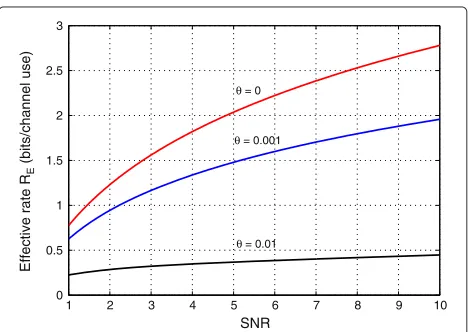
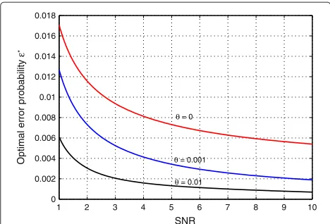
Finally, we provide numerical results for the optimal effective rate and optimal error probability as a func-tion of SNR in Figures 6 and 7, respectively, for θ =
0, 0.001, and 0.01. We see that for fixed θ, increas-ing the SNR improves the throughput and also the reliability of the transmissions by lowering the error probabilities.
5 The impact of different transmission strategies Heretofore, we have considered the scenario where the transmitter knows the fading coefficients {hi} and per-forms variable-rate transmission with the same average power P in each coherence block of m channel uses. Next, we investigate the throughput achieved with other transmission strategies such as employing power control, transmitting data at fixed rates, and sending independent messages over two parallel channels.
1 2 3 4 5 6 7 8 9 10 0
0.5 1 1.5 2 2.5 3
SNR
Effective rate R
E
(bits/channel use)
θ = 0
θ = 0.001
θ = 0.01
Figure 6The optimal effective rateREvs. SNR in the Rayleigh
1 2 3 4 5 6 7 8 9 10 0
0.002 0.004 0.006 0.008 0.01 0.012 0.014 0.016 0.018
SNR
Optimal error probability
ε
*
θ = 0
θ = 0.001
θ = 0.01
Figure 7The optimal error probability∗vs. SNR.The blocklength ism=1, 000.
5.1 Power control
In this subsection, we investigate the gains achieved by varying the transmission power as well with respect to fading. Let us denote the power adaptation normalized by the noise power byμ(SNR,θ,|h|2). With this adaptation
policy, the transmission rate is
¯
r=log2 1+μ SNR,θ,|h|2|h|2
−
1
m
1− 1
μ SNR,θ,|h|2|h|2+12
Q−1()log2e
(18)
which is obtained by replacing SNR withμ(SNR,θ,|h|2)
in (11). Finding the optimal power adaptation policy that maximizes ¯r or the effective rate RE(θ ) = −m1θ logeE|h|2
+(1−)e−θm¯ris in general a difficult task
due to the facts that both the first and second terms on the right-hand side of (18) are concave functions. Hence, ¯
ris neither concave nor convex. For this reason, we resort to suboptimal strategies. One viable policy,μ∗, is the one that maximizes the effective rate when the service pro-cess is assumed to be equal to the instantaneous capacity log(1+μ(SNR,θ,|h|2)|h|2)with zero error probability, i.e.,
μ∗ SNR,θ,|h|2=arg max
E|h|2{μ(SNR,θ,|h|2)}≤SNR
− 1 mθ
×logeE|h|2
e−θmlog2(1+μ(SNR,θ,|h|2)|h|2)
. (19)
μ∗is derived in [2] and is given by
μ∗ SNR,θ,|h|2} =
1
αβ+11(|h|2)
β β+1
− 1
|h|2 |h|2≥α
0 |h|2< α,
(20)
where β= logθm
e2, and α is chosen such that the
average long-term signal-to-noise ratio constraint,
E|h|2{μ(SNR,θ,|h|2)} ≤ SNR, is satisfied with
equal-ity. Note that this policy is close to the optimal one when the blocklength is large, and hence, r¯ is close to log(1+μ(SNR,θ,|h|2)|h|2), andis close to zero.
In Figure 8, the optimal effective rate is plotted as a function of θ for both fixed- and variable-power cases. In the fixed-power case, SNR = 0 dB in each coherence block. When power adaptation is employed, signal-to-noise ratioμ(SNR,θ,|h|2)varies in each block while satis-fyingE|h|2{μ(SNR,θ,|h|2)} ≤SNR=0 dB. The improved
performance with power control is observed in the figure.
5.2 Fixed-rate transmissions
The analysis so far has assumed that the transmitter has perfect knowledge of the fading coefficients and can perform variable-rate and/or variable-power trans-missions in each coherence block. On the other hand, it is practically interesting to consider cases in which the transmitter does not know the channel and send the information at a fixed rate. Additionally, the trans-mitter may prefer fixed-rate transmissions, even when it knows the channel, due to complexities in varying the transmission rate for each block. Motivated by these considerations, we assume in this section that the trans-mitter sends the information at the fixed rate¯rf. Under
this assumption, error probability varies with the fad-ing realizations. The analysis in the previous sections have, on the other hand, considered the scenarios in which the error probability is fixed for all channel states.
From (11), which provides the fundamental tradeoff between the rate and error probability in the finite
block-0 0.02 0.04 0.06 0.08 0.1 0
0.1 0.2 0.3 0.4 0.5 0.6 0.7
θ
Effective rate R
E
(bits/channel use)
with power control
fixed power
Figure 8Optimal effective rateREvs. QoS exponentθin
length regime, we can easily see that the error probability
Note that is a function of the fading magnitude|h|,
signal-to-noise ratio SNR, and blocklengthm. The service rate (in bits permchannel uses) is now
Ri= It can also be immediately seen that for given SNR, blocklength m, QoS exponent θ, and fixed-rate rf, the
effective rate in bits per channel use is
RE(θ )= −
1
mθ logeE|h|2
+(1−)e−θm¯rf (23)
which is essentially the same as in (13). The only difference is that we now have the rate fixed and error probability varying. Similarly, whenθ =0, we have
RE(0)=E|h|2{(1−)rf¯ } =(1−E|h|2{})rf¯
It is instructive to investigate what is obtained asm →
∞. We immediately see that
lim
which is defined as the capacity with outage ([19], Section 4.2.3). Therefore,RE(0)in (24) can be seen as the outage
capacity in the finite blocklength regime. Furthermore,
RE(θ ) in (23) can be regarded as the generalization of
such a throughput measure to the scenario with QoS limitations.
In Figures 9, 10, and 11, we illustrate the numerical results. In Figure 9, the effective rate is given as a func-tion of the fixed transmission rater¯f. We observe that the
effective rate curves are quasiconcave; moreover, they are maximized at a unique value ofr¯f. We also observe that
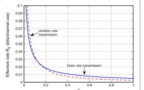
the maximum value of the effective rate diminishes with increasingθ. This is more clearly seen in Figure 10, where the optimal effective rates (optimized over r¯f) are
plot-ted as a function ofθ. In this figure, we have curves for both fixed-rate and variable-rate transmissions. The effec-tive rate for the variable-rate transmission is computed by maximizing (13) over. It is interesting to observe that the fixed-rate transmissions perform worse than variable-rate transmissions for small values ofθ. However, forθ >0.13, the fixed-rate transmissions start outperforming. Hence, for high enough values ofθ, fixing the transmission rate and having the error probability vary in each block provide better performance than requiring the error probability to be fixed by varying the rate. Additionally, though not treated in this paper, another strategy in which both the error probability and transmission rate adapt and vary with the fading can bring forth improvements in the per-formance. Finally, in Figure 11, we note that asθincreases, the optimal fixed rate¯rf, which maximizesRE(θ )in (23),
diminishes.
5.3 Sending independent messages over two parallel channels
Up until now, we have assumed that the transmitter sends a single codewordx = [xr xi] of length 2minm
chan-nel uses. Another approach is to transmit two indepen-dent messages using codewordsxr andxi selected from
0 1 2 3 4 5
(bits/channel use)
θ = 0.001
θ = 0
θ = 0.01
θ = 0.1
Figure 9Effective rateREvs. the fixed transmission rate¯rfin the
Rayleigh fading channel.SNR=0 dB, and the blocklength is
0 0.2 0.4 0.6 0.8 1
(bits/channel use)
variable−rate transmission
fixed−rate transmission
Figure 10Optimal effective rateREvs.θin Rayleigh fading for
variable-rate and fixed-rate transmissions.SNR=0 dB, and the blocklength ism=1, 000.
two independent codebooks. Note that, now, the code-word length is m. These two independent codewords can be seen to be sent through two independent parallel channels:
Since the blocklength ismfor each codeword, the trans-mitter sends the information through each channel in the
ith block duration at the following rate with block error probability:
where the subscriptp is introduced to differentiate this rate from that in (11). Since errors occur independently in each channel, the service rate (in bits permchannel uses) in each block duration ofmchannel uses is
Ri=
When the transmitter sends two independent messages over the independent real and imaginary channels, the effective rate in bits per channel use at a given SNR,
0 0.2 0.4 0.6 0.8 1
Figure 11The optimal fixed transmission rate¯rfvs. QoS exponentθin the Rayleigh fading channel.SNR=0 dB, and the blocklength ism=1, 000.
error probability , blocklength m, and QoS exponent
θis whererpis given in (29).
In this case, it can again be easily shown that the error probability that maximizes the effective rate in (32) is unique. The following is a corollary to Proposition 1.
Corollary 1.Assume that the values of m,θ > 0, and SNR>0are fixed. Then, the function
p()=E|h|2
(+(1−)e−θm¯rp)2
(33)
is strictly convex in, and therefore, the optimal value of that minimizes this function or equivalently maximizes the effective rate in (32) is unique. Moreover, REin (32) is a
quasiconcave function of.
Proof.See Appendix 3.
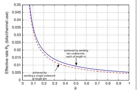
which can immediately be seen to be smaller than the effective rate in (15). Hence, whenθ =0, using two code-words, each of lengthmprovides lower throughput than using a single codeword of length 2m. On the other hand, as we observe in Figure 12, the throughput achieved by sending two codewords is higher ifθ increases beyond a threshold. Therefore, under strict QoS constraints, send-ing in each coherence block multiple codewords with shorter lengths may be preferable.
6 Conclusion
We have analyzed the performance of buffer-constrained wireless systems in the practical scenario in which trans-missions are performed using finite blocklength codes with possible decoding errors at the receiver. Employing a recent result on coding rate in the finite blocklength regime, we have determined the effective rate expression as a function of the QoS exponent, coding blocklength, decoding error probability, and signal-to-noise ratio, and characterized the throughput under statistical QoS con-straints. We have discussed different transmission strate-gies. In the case in which the transmission rate is varied and the error probability is kept fixed across different fading realizations, we have shown that the effective rate is maximized at a unique error probability. This opti-mal decoding error probability gives us insight on the required reliability of the channel codes. Through numer-ical results, we have investigated how the optimal effective rate and optimal error probability vary with the QoS expo-nentθ. We have also had interesting observations on the performance as a function of the blocklength. We have analyzed the throughput improvements through power adaptation. We have studied the practical scenario in which the transmitter sends the information at a fixed transmission rate. We have seen that while variable-rate
0 0.1 0.2 0.3 0.4 0.5 0.6 0.7 0.8 0.9 1 0
0.005 0.01 0.015 0.02 0.025 0.03 0.035 0.04 0.045 0.05
θ
Effective rate R
E
(bits/channel use)
achieved by sending two codewords, each of length m
achieved by sending a single codeword
of length 2m
Figure 12The optimal effective rateREvs.θin the Rayleigh
fading channel.SNR=0 dB, and the blocklength ism=1, 000. The dashed curve is the effective rate in (13) maximized over, and the solid curve is the effective rate in (32) maximized over.
schemes provide higher effective rate at low values of
θ, fixed-rate transmissions start performing better as θ
increases. Finally, we have noted that sending multiple codewords with shorter blocklengths in each coherence interval can become a favorable strategy under stringent QoS constraints.
Endnotes
aFor time-varying arrival rates, effective capacity
specifies the effective bandwidth of the arrival process that can be supported by the channel.
bNote that multiplication of the channel output with e−jθhjust rotates the output, is a reversible operation, and
hence does not lead to any loss of information.
cThe interchange of the limit and the integral (or
equivalently the expectation) can be easily justified by noting the boundedness of theQ-function, i.e., |Q(·)| ≤1, and invoking the dominated convergence theorem. Additionally, we implicitly assume that the random variable log2(1+SNR|h|2)does not have a mass atr¯f; hence,r¯f =log2(1+SNR|h|2)is a zero-probability
event, and this event does not affect the expectation.
Appendices
Appendix 1: Proof of Proposition 1 We first prove the following Lemma.
Lemma 1. For fixed m, SNR>0, and|h|2>0,
f()=(1−)e−θm¯r (36)
is a strictly convex function of.
Proof. We first express
−θmr¯=aQ−1()+b (37)
where, from (11),
a=θ
m
1− 1
(SNR|h|2+1)2
loge and
b= −θmlog2(1+SNR|h|2). (38)
Note that since SNR> 0,|h|2 >0, andθ > 0, we have
a>0. With the above definitions, we can write
f()=(1−)eaQ−1()+b. (39)
The first and second derivatives off()with respect to
can easily be found as follows: ˙
f()=a(1−)Q˙−1()−1eaQ−1()+b (40) ¨
f()=a(1−)(Q˙−1())2−2Q˙−1()
to prove the lemma. Note that for an invertible and dif-ferentiable function g, we have g(g−1(x)) = x. Taking derivative of both sides of this equality leads us to
˙
g−1(x)= 1
˙
g(g−1(x)), (42)
whereg˙−1(x)denotes the derivative ofg−1with respect to
x, andg(g˙ −1(x))is the derivative ofgevaluated atg−1(x). Following this approach and noting that
Q(x)=
, ∞
x
1 √
2π e −t2/2
dt, and
˙
Q(x)= −√1
2πe −x2/2
, (43)
we can easily find the following expression:
˙
Q−1()= −√2πe(Q −1())2
2 . (44)
Note thatQ˙−1() <0 for any 0≤ ≤1. Differentiating ˙
Q−1()with respect to, we obtain the second derivative as follows:
¨
Q−1()=2πQ−1()e(Q−1())2. (45)
Next, we consider two cases:
(1) <1/2. First, we assume that <1/2. Under this assumption, we haveQ−1() >0and hence
¨
Q−1() >0. Together with the fact thatQ˙−1() <0, we immediately see that
¨
f() >0 for <1/2. (46)
(2) >1/2. Next, we analyze the case in which >1/2 and thereforeQ−1() <0. We concentrate on the term inside the square parentheses in (41). Using (44) and (45), and definingx=Q−1()or equivalently Q(x)=, we can write
a(1−)(Q˙−1())2−2Q˙−1()+(1−)Q¨−1()
(47) =a(1−)2πe(Q−1())2+2√2πe(Q−1())2/2
+(1−)2πQ−1()e(Q−1())2 (48) =a(1−Q(x))2πex2 +2√2πex2/2
+(1−Q(x))2πxex2 (49)
=ex2/2
2π(1−Q(x))(x+a)ex2/2+2√2π
(50) ≥ex2/2
2π(1−Q(x))xex2/2+2√2π
(51)
≥ex2/2
2π√ 1
2π (−x)e −x2/2
xex2/2+2√2π
(52) ≥ex2/2−√2π+2√2π
(53)
≥ex2/2
√
2π
>0. (54)
Above, (51) follows from the fact thata> 0 and hence
x+a>x. (52) is obtained by using the upper bound,
1−Q(x)=Q(−x) < √ 1
2π (−x)e −x2/2
forx<0, (55)
and recognizing that by our assumptionx = Q−1() <
0, and(1−Q(x))is multiplied above byx < 0, enabling us to find a lower bound. From the above discussion, we conclude that
¨
f() >0 for >1/2. (56)
Finally, note that when = 1/2 and henceQ−1() =
Q−1(1/2)=0, we have
a(1−)(Q˙−1())2−2Q˙−1()+(1−)Q¨−1() (57) =a(1−)2πe(Q−1())2
+2√2πe(Q−1())2/2+(1−)2πQ−1()e(Q−1())2
(58)
=aπ+2√2π >0, (59)
and thereforef¨(1/2) >0. Sincef¨() >0 for all ∈[0, 1],
f()is a strictly convex function of. We now define
ψ ()=+f()=+(1−)e−θm¯r (60)
which is also strictly convex as it can be immediately seen that ψ ()¨ = ¨f(e) > 0 for SNR > 0 and |h|2 > 0. Note that if eitherSNR = 0 or|h|2 = 0, the coding rate
becomes¯r= 0, leading toψ ()=1. Since the nonnega-tive weighted sum (including infinite sums and integrals) of strictly convex functions is strictly convex ([20], Section 3.2.1) and since the addition of a constant (in the case of |h|2=0) does not have an impact on the strict convexity, we immediately conclude that
()=E|h|2{ψ ()} =E|h|2
+(1−)e−θm¯r (61)
Finally, we address the quasiconcavity of the effective rate
RE(θ,)= −
1
mθ logeE|h|2
+(1−)e−θm¯r
= − 1
mθ loge() (62)
with respect to. A functionf is quasiconvex if and only iff(δx+(1−δ)y) ≤ max{f(x),f(y)}for anyδ ∈ [0, 1], and the negative of a quasiconvex function is quasiconcave [20]. Now, we can easily show for any1,2 ∈ (0, 1)and
δ∈[0, 1] that
−RE(θ,δ1+(1−δ)2)=
1
mθ loge(δ1+(1−δ)2)
≤ 1
mθ loge
δ(1)+(1−δ)(2)
(63)
≤ 1
mθ loge
max{(1),(2)}
(64)
=max
1
mθ loge(1),
× 1
mθ loge(2)
*
(65)
=max{−RE(θ,1),−RE(θ,2)}
(66)
where the inequality in (63) is obtained from the facts that
is a convex function and hence(δ1+(1−δ)2) ≤ δ(1) + (1 − δ)(2), and logarithm is a monotoni-cally increasing function; (64) follows from the inequality
δ(1)+(1−δ)(2)≤ max{(1),(2)}; and (65) is
again due to the monotonicity of the logarithm. Therefore, −RE is quasiconvex and RE is a quasiconcave function
of.
Appendix 2: Proof of Proposition 2
Proof. The proof is similar to that of Proposition 1 in Appendix 1 and will be kept brief. Let us first consider the function
φ ()=(1−)¯r=(1−) c1−c2Q−1()
, (67)
where we define c1 = log2(1 + SNR|h|2) and c2 =
1
m
1− (SNR|h|12+1)2loge. Note that if either SNR = 0
or|h|2=0, thenc
1=c2=0 andφ ()=0 for all. Next,
we consider the case in which SNR>0 and|h|2>0, and
thereforec1 > 0 andc2 > 0d. The second derivative of
φ ()with respect tois
¨
φ()=2c2Q˙−1()+c2(−1)Q¨−1(). (68)
Using similar arguments as in Appendix 1, we can easily see that for <1/2,φ() <¨ 0. For >1/2, we can show, employing the steps similar to those in (47) to (54), that
¨
φ() <−c2
√
2πex2/2<0, (69)
where x = Q−1(). When = 1/2, we have φ()¨ =
−2√2πc2 < 0. Sinceφ() <¨ 0 for all,φ ()is a strictly
concave function of when |h|2 > 0 and SNR > 0. As argued similarly in Appendix 1, since the nonnega-tive weighted sum of strictly concave functions is strictly concave [20], and since the addition of a constant (in the case of |h|2 = 0) does not have an impact on the strict concavity, we conclude that
RE(0)=(1−)E|h|2{¯r} =(1−)E|h|2{ c1−c2Q−1()}
=E|h|2{φ ()} (70)
is a strictly concave function of.
Appendix 3: Proof of Corollary 1
Proof. From the proof of Proposition 1 in Appendix 1, it immediately follows that+(1−)e−θm¯rpis a strictly
convex function of. Then,(+(1−)e−θm¯rp)2is strictly
convex due to the facts thatf(x) =x2is a strictly convex and increasing function ofxand the compositionf(g(x))
is strictly convex function wheng(x) is a strictly convex function ([20], Section 3.2.4). Then, the strict convexity ofE|h|2
(+(1−)e−θm¯rp)2and quasiconcavity of the
effective rate follow from the arguments employed at the end of Appendix 1.
Competing interests
The author declares that he has no competing interests.
Acknowledgements
This work was supported by the National Science Foundation under grants CCF – 0546384 (CAREER), CNS – 0834753, and CCF-0917265. The material in this paper was presented in part at the 2011 IEEE International Conference on Communications (ICC), Kyoto, Japan.
Received: 24 April 2013 Accepted: 29 October 2013 Published: 21 December 2013
References
1. D Wu, R Negi, Effective capacity: a wireless link model for support of quality of service. IEEE Trans. Wireless Commun.2(4), 630–643 (2003) 2. J Tang, X Zhang, Quality-of-service driven power and rate adaptation over
wireless links. IEEE Trans. Wireless Commun.6(8), 3058–3068 (2007) 3. J Tang, X Zhang, Quality-of-service driven power and rate adaptation for
multichannel communications over wireless links. IEEE Trans. Wireless Commun.6(12), 4349–4360 (2007)
4. J Tang, X Zhang, Cross-layer-model based adaptive resource allocation for statistical QoS guarantees in mobile wireless networks. IEEE Trans. Wireless Commun.7, 2318–2328 (2008)
5. L Liu, P Parag, J Tang, W-Y Chen, J-F Chamberland, Resource allocation and quality of service evaluation for wireless communication systems using fluid models. IEEE Trans. Inform. Theory53(5), 1767–1777 (2007) 6. P L Liu, J-F Parag, Chamberland, Quality of service analysis for wireless
7. MC Gursoy, D Qiao, S Velipasalar, Analysis of energy efficiency in fading channel under QoS constrains. IEEE Trans. Wireless Commun.
8(8), 4252–4263 (2009)
8. D Qiao, MC Gursoy, S Velipasalar, The impact of QoS constraints on the energy efficiency of fixed-rate wireless transmissions. IEEE Trans. Wireless Commun.8(12), 5957–5969 (2009)
9. D Qiao, MC Gursoy, S Velipasalar. Energy efficiency of fixed-rate wireless transmissions under queueing constraints and channel uncertainty. Paper presented at the IEEE Global Telecommunications Conference (GLOBECOM) (Honolulu, HI, 30 Nov–4 Dec 2009)
10. R Negi, S Goel. An information-theoretic approach to queuing in wireless channels with large delay bounds. Paper presented at the IEEE Global Telecommunications Conference (GLOBECOM) (Dallas, TX , USA, 29 Nov–3 Dec 2004)
11. S Goel, R Negi. Analysis of delay statistics for the queued-code. Paper presented at the IEEE International Conference on Communications (ICC) (Dresden, Germany, 14–18 Jun 2009)
12. Y Polyanskiy, HV Poor, S Verdú, Channel coding rate in the finite blocklength regime. IEEE Trans. Inform. Theory56(5), 2307–2359 (2010) 13. JN Laneman. On the distribution of mutual information. Paper presented
at the Workshop on Information Theory Applications (ITA) (San Diego, CA, USA, 13 Feb 2006)
14. D Buckingham, MC Valenti. The information-outage probability of finite-length codes over AWGN channels. Paper presented at the 42nd Annual Conference on Information Sciences and Systems (CISS) (Princeton, NJ, USA, 19–21 Mar 2008)
15. P Wu, N Jindal, Coding versus ARQ in fading channels: how reliable should the PHY be? IEEE Trans. Commun.59(12), 3363–3374 (2009) 16. C-S Chang, T Zajic. Effective bandwidths of departure processes from
queues with time varying capacities. Paper presented at the IEEE INFOCOM (Boston, MA, USA, 2–6 Apr 1995)
17. C-S Chang, Stability, queue length, and delay of deterministic and stochastic queuing networks. IEEE Trans. Auto. Control
39(5), 913–931 (1994)
18. C-S Chang,Performance Guarantees in Communication Networks. (Springer, New York, 1995)
19. A Goldsmith,Wireless Communications. (Cambridge University Press, Cambridge, 2005)
20. S Boyd, L Vandenberghe,Convex Optimization. (Cambridge University Press, Cambridge, 2004)
doi:10.1186/1687-1499-2013-290
Cite this article as:Gursoy:Throughput analysis of buffer-constrained wireless systems in the finite blocklength regime.EURASIP Journal on Wireless Communications and Networking20132013:290.
Submit your manuscript to a
journal and benefi t from:
7Convenient online submission 7Rigorous peer review
7Immediate publication on acceptance 7Open access: articles freely available online 7High visibility within the fi eld
7Retaining the copyright to your article