R E S E A R C H
Open Access
Air quality forecasting based on cloud
model granulation
Yi Lin
1, Long Zhao
3, Haiyan Li
4and Yu Sun
2*Abstract
This paper proposes a novel algorithm based on cloud model granulation (CMG) for air quality forecasting. Through data exploration of three different types of monitoring localities in Wuhan City, the determinative pollutants were reduced to NO2, PM10, O3, and PM25for modeling. After iterative granulation of original time series, the concepts of cloud model were extracted for each granule from original data space to feature space. Then, the cloud model features of future granules were predicted in the new feature space. Finally, the value in the feature space is transformed into the solution in the concept space. In addition, this paper uses the grid search to optimize the parameters in all experiments. Compare with several machine learning approaches, considering the mean squared error, the results on composition model and direct model shows that the proposed algorithm has better in predicting both individual air quality index and air quality index. At ZKX locality, the CMG algorithm can achieve high accuracy 71.43% for prediction of air quality index class. The results show that this algorithm not only can simplify the modeling process of uncertain time series in the form of knowledge abstraction, but also has good prediction performance in IAQI and AQI.
Keywords:Cloud model, Soft computing, Machine learning, Uncertainty, Air quality forecasting
1 Introduction
In health issues related to deterioration of air quality, people use air quality index (AQI) [1–3] to report on the conditions of air pollutants (APs), which were first pro-posed and universally acknowledged as one important de-terminant of adverse health effects. In the Aphekom project, the paper [4] pointed out that a reduction in APs would bring significant health and currency benefits to Europe. Recently, more and more researchers have paid attention to air quality forecasting (AQF). Previous litera-ture has shown that the air quality forecasting is a com-plex problem, whose relevant data are non-linear, uncertain, and heterogeneous. Therefore, the soft comput-ing (SC) and machine learncomput-ing (ML) approaches can pro-vide good results [1, 5–7]. When attempting to design a model combined with several APs, the problem may be-come more complex. Only very few attempts have been made to solve this issue [1, 8, 9]. Unfortunately, these models lost a lot of information because it converted the values of AQIs to nominal values for classification tasks.
So far, all the literature on AQF can be divided into three categories [10]: (1) simple empirical methods, (2) physically based methods, and (3) parametric or non-parametric statistical methods. In simple empirical methods, there are two ways to predict tomorrow’s value: (1) using present day’s value (persistence method) (2) relying critically on the dependencies between me-teorological variables and predicted air pollutants. Either way, it provides low prediction accuracy. The physically based approaches model the temporal and spatial pat-terns of APs and meteorological variables [11], which are more accurate than the simple empirical methods. In fact, these processes are too usually too complex to be represented with physically based models. Therefore, such models can lead to biased predictions. Parametric or non-parametric statistical approaches [12, 13] can be superior to outperform physically based approaches in prediction accuracy [14], such as neural networks (NNs). However, there are some disadvantages of artificial intelligence approaches reported in the current research on APs prediction [6, 15]. Firstly, because these models are developed under meteorological conditions and chemical of some specific localities, it cannot be employed in other areas. Secondly, these models usually * Correspondence:[email protected]
2School of Computer and Electronics and Information, Guangxi University,
Nanning, China
Full list of author information is available at the end of the article
simplify the meteorological process. Thirdly, the interre-lationships among multiple pollutants are not modeled.
Zhang et al. [10] have shown that the NNs models give significantly higher accuracy than the linear regression approaches in the prediction of future AP concentra-tions, because it can model the complicated non-linear relationships between independent variables and object-ive functions. Recently, the support vector regression (SVR) [16] has been proven to perform better or equal than NNs in a variety of APs’ predictions [17]. Com-pared with many other methods, such as NNs, SVR has obvious dominance. The former minimizes empirical risk and the latter minimizes structural risk. Therefore, the SVR model is relatively insensitive to the limited number of train data, and the error of test data is also limited by the SVR model. That is, the SVR model has stronger generalization performance. Lately, the fuzzy logic-based models [1, 5, 18] have been used to predict APs, which were capable of processing the inherent un-certainties in both human knowledge and data. But these approaches may suffer from computational complexity, and their prediction accuracy is lower than SVR [1].
The purpose of this study is to design one algorithm for air quality forecasting which could accommodate the un-certainties in the data at lower computational cost and good generalization performance. This algorithm not only considers the fuzziness and randomness of the problem as a whole, but also through transformation of three different state space to reduce data. First, the time series in the ori-ginal data space is iteratively granulation and mapped into the new granules time series in the feature space. Then, the cloud model feature of each granule is extracted and deductive reasoning is performed. Finally, from the feature data space to the concept space, the proposed algorithm solves the original problem based on the task to be solved and the related knowledge. In addition, the paper uses the grid search to optimize all the parameters in the experi-ments. The results show that the proposed algorithm is capable of (1) modeling the uncertainties between data sampling points of time series; (2) maximizing generalization performance; (3) and finally costing lower computational cost.
In our study, it conducted contrast experiments at three different regions of Wuhan City. First of all, it per-forms data exploration to grasp the features of target data. Next, it gives the proposed algorithm’s detailed de-scription and explanation, which has also not been reported in the literature so far. Additionally, it com-pares this approach with several popular algorithms, non-linear autoregressive neural networks (NARNNs) [19] and SVR, on the prediction of IAQI and AQI time series. The results suggest that the CMG algorithm ob-tains better or nearly performance than contrast algo-rithms in the most experiments. At ZKX, the proposed
algorithm can achieve high accuracy 71.43% on the pre-diction of AQI class. In the future, the research will focus on the quantitative calculation between fuzzy and random of the cloud model, and it hopes to give the value range of the problem to be solved according to the specified degree of certainty, which also can be used for other problems with uncertainty.
2 Methods
2.1 Air quality forecasting
The datasets of our studies were come from the Wuhan Municipal Environmental Protection Bureau, which con-tain the information about maximum daily emission var-iables(SO2, NO2, PM10, CO, O3, PM2.5) and other knowledge (primary pollutants, Air quality index, AQI index class) from three localities in 2016~ 2017: Ganghua of Qingshan District (GH), south area of Jianghan District (JHS), and new area of Zhuankou locality (ZKX).The basic information about these studied localities is provided as follows: Ganghua locality is an urban residential zone, localized at 30°37′34.60″ north latitude, 114°22′11.13″ east longitude, altitude = 26 m; south area of Jianghan locality (JHS) is an urban com-mercial zone, localized at 30°18′38.86″ north latitude, 114°05′9.13″ east longitude, altitude = 16 m; new area of Zhuankou locality (ZKX) is an urban industrial zone, localized at 30°28′57.89″ north latitude, 114°09′ 24.07″east longitude.
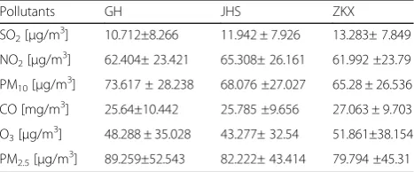
As presented in Table 1, there are six maximum daily emission variables, including SO2, NO2, PM10, CO, O3, PM2.5, for individual localities GH, JHS, and ZK. The JHS locality has the best air quality, while the GH local-ity, in particular, showed high levels of PM10 and PM2.5, and the ZKX locality, in particular, showed high levels of O3. This is because the characteristics of the zones de-termined the air quality to a great extent [1].
After data statistical, it is not difficult to find that there is about 1.93% of data is missing. In order to improve the accuracy of air quality forecasting, there are usually three approaches to deal with missing data before mod-eling: (1) deleting sample instances with missing data; (2) replacing missing values; and (3) using multiple im-putations. The most common way is to replace the
Table 1Basic descriptive statistics (mean ± StdDev) of monitored pollutants
Pollutants GH JHS ZKX
SO2[μg/m 3
] 10.712±8.266 11.942 ± 7.926 13.283± 7.849
NO2[μg/m 3
] 62.404± 23.421 65.308± 26.161 61.992 ±23.79
PM10[μg/m 3
] 73.617 ± 28.238 68.076 ±27.027 65.28 ± 26.536
CO [mg/m3] 25.64±10.442 25.785 ±9.656 27.063 ± 9.703
O3[μg/m 3
] 48.288 ± 35.028 43.277± 32.54 51.861±38.154
PM2.5[μg/m 3
missing value by selecting the reasonable value based on the context of the problem. In this way, it does not need to delete any sample instances. That is, this method does not lose any information but may lead to slightly biased estimates. In this paper, it uses the mean instead of miss-ing values for numeric attribute and the most for nom-inal attributes.
In this study, the individual air quality index (IAQI) refers to the air quality index calculated according to the concentration of individual pollutant, whose formula is expressed as follows:
IAQIi¼CIhigh−Ilow
high−Clow
Ci−Clow
ð Þ þIlow ð1Þ
Where Ci is the pollutant concentration of APi, Clow denotes the nearest concentration breakpoint that is ≤C, Chighdenotes the nearest concentration breakpoint that is
≥C, Ilowindicates the index breakpoint corresponding to ClowandIhighindicates the index breakpoint correspond-ing to Chigh. So, the IAQI formula is purely based on piecewise linear function using pollutant concentration breakpoints. In this way, the total daily health impact is expected to be the sum of the values associated with each AP [20]. In addition, the measurement intervals of these six pollutants were not identical to each other in China. For example, the concentration of PM2.5 and PM10 are measured by the average of the last 24 h. SO2, NO2, O3, CO are measured by the average of last hour. It is remark-able that this approach for computing AQI is different from the way used in Europe [1, 21]. Because the latter uses AQIs for the city’s background and traffic conditions, it emphasizes on the role as a traffic pollutions sources.
The air quality indexes of Ministry of Environmental Protection (MEP) in China were used as target variables in this study. According to the formula published by the MEP [22], the AQI is expressed as follows:
AQI¼ max IAQIð 1;IAQI2;…;IAQInÞ ð2Þ
where IAQIi is the individual air quality index value for
the i-th air pollutant, i= 1, 2, …, n and n denote the number of air pollutants. It is obvious that this approach uses only the maximum value of IAQI to calculate the value of AQI. In this formula, the effects of each AP are independent, without considering the interaction be-tween of different APs. The daily maximum concentra-tion limits of the examined air pollutants were published by China MEP as follows: SO2: 2620 μg/m3, NO2:
940 μg/m3, PM10: 600 μg/m3, CO: 60 mg/m3, O3:
1200 μg/m3. While the pollutant concentration exceeds the upper limit, the maximum value of IAQI is still 500. The value beyond the maximum index is not available. In this case, it named “Beyond Index”[22]. It should be noted that the concentration limits of different air
pollutants items are different from regional types and time scales. In general, the timescales are longer, the concentration limit is lower; the concentration limits of the first districts, such as nature reserves, scenic areas, and other areas requiring that need special protection, are lower than those of the second districts such as residential areas, commercial transportation, mixed residential areas, cultural areas, industrial areas, and rural areas.
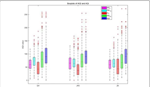
As shown in Fig. 1, the boxplots depict the general span of IAQI (NO2, PM10, O3, PM25) and the AQIs in above three localities. It is not difficult to find that, the IAQI and AQI in GH locality were generally higher than other two localities. The JHS locality showed higher NO2 and the ZKX locality showed higher O3. In JHS locality, the AQIs were significantly lower than other two localities. The distribution range of the IAQIs and AQIs in the GH and JHS localities were similar.
In life, what people pay more attention to is the AQI class. It is more concise, intuitive, and easy to under-stand than AQIs. According to technical regulation on ambient air quality index [22], the AQIs were further transformed into six classes as shown in Table2.
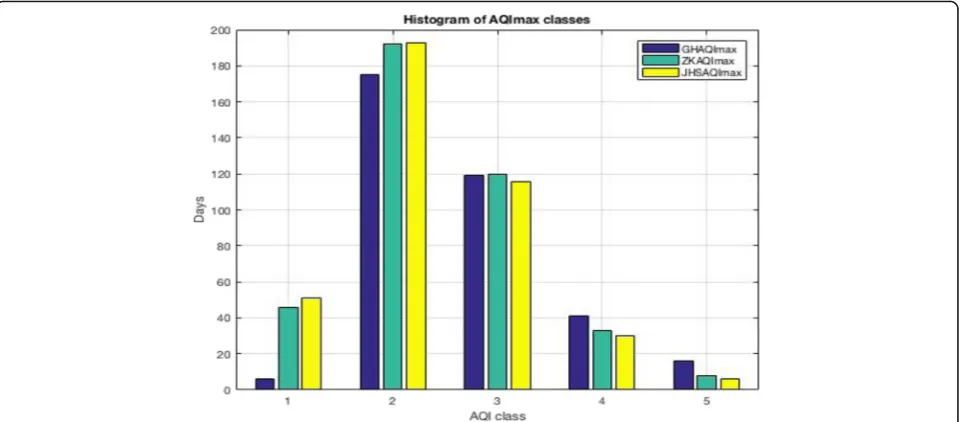
Figure2computes the cumulative days of various diffe-rent air quality classes at diffediffe-rent localities in the observa-tion period, which shows further detailed informaobserva-tion on the distribution of the AQI classes. The AQIs show that the air in these localities is good or slightly polluted.
Figure 3 provides the composition and percentages of determinative pollutants in the AQIs. It is found that PM2.
5and O3play a determining role in the AQI computing, while NO2and SO2together account for about 20~ 30% importance. The impacts degree of determinative pollut-ants was calculated in the occurrence proportion of AQI.
2.2 Algorithm based on cloud model granulation
Recent studies show that NNs and SVR have achieved significant improvement compared to the previous methods in the prediction of APs [12]. But the data of APs are non-linear, heterogeneous, and uncertain. The fuzzy logic systems have an advantage in dealing with the inhe-rent uncertainty of data and human cognition, which suf-fer from computational cost. In this paper, it proposed an method based on concept extraction of cloud model and the conversion of state space on time series prediction of APs and AQI. This method can not only in processing un-certainty at coarser granularity, but also take into account both efficiency and generalization performance.
In 1995, the cloud model was first proposed by Deyi Li [26], who is a member of Chinese Academy of Engineering. The cloud model is a model of mutual conversion between qualitative concepts and quantitative descriptions. It has been applied in many fields, such as intelligent evaluation and fuzzy assessment. The cloud model integrates the probability theory and fuzzy set theory. By constructing a specific algorithm, the randomness, fuzziness, and rele-vance between concepts are unified. Cloud model does not require a priori knowledge, which can analyze the statis-tical rules from a large number of raw data and realize the transformation from quantitative value to the qualitative concept. It has three digital features: expectation Ex,
Table 2AQI classes of China’s Ministry of Environmental Protection
Range AQI class Class description
0–50 1 Excellent, no health implications.
51–100 2 Good, few hypersensitive individuals should reduce outdoor exercise.
101–150 3 Slight pollution, slight irritations may occur, individuals with breathing or heart problems should reduce outdoor exercise.
151–200 4 Moderate pollution, slight irritations may occur, individuals with breathing or heart problems should reduce outdoor exercise.
201–300 5 Heavy pollution, healthy people will be affected significantly. People with breathing or heart problems will experience reduced endurance in activities. These individuals and elders should remain indoors and restrict activities.
300+ 6 Severe pollution, the endurance of healthy people in activities will decrease. There may be strong irritation symptoms that may cause other diseases. The old and the sick should stay indoors to avoid exercise. Healthy should avoid outdoor activities.
Fig. 1Boxplots of IAQI and AQI. The boxplots depict the general span of IAQI (NO2, PM10, O3, PM25) and the AQIs in above three localities. The
entropy En, and super entropy He, which reflects the over-all features of qualitative concepts. Expectation Ex is the most representative value of the qualitative concept in the domain space. Entropy En reflects the range of number domains that can be accepted by the concept. Hyper Entropy He is the measure of entropy’s uncertainty, that is entropy’s entropy.
In the process of human cognitive thinking, the con-cepts are relative and hierarchical. Concon-cepts or values of the same attribute usually belong to more than one upper-class concept. The proposed algorithm abstracts the target time series into mutually overlapping
conceptual granules sequences then predicts them by in-ference judgment of qualitative concept extension. Each concept is one basic information granule, and the time range of information covered by each concept is called the window width of the granule. By backward cloud gener-ator [27,28], the proposed algorithm converts the distri-bution characteristics of data samples in each granlue into qualitative concepts represented by three digital features exception Ex, entropy En, and hyper entropy He.
After extracting concept features of the cloud model, SVR is used to predict the feature sequences Ex, En, and He respectively. The greater the probability of cloud Fig. 2Histogram of AQI classes. It computes the cumulative days of various different air quality classes at different localities in the observation period. The first group of histograms shows the days that belong to the first AQI class at three locations. The second group of histograms shows the days that belong to the second AQI class at three locations. The third group of histograms shows the days that belong to the third AQI class at three locations. The fourth group of histograms shows the days that belong to the fourth AQI class at three locations. The fifth group of histograms shows the days that belong to the fifth AQI class at three locations. The blue column is the result of the GH locality and the green column is the result of the ZKX locality. The yellow column is the result of the JHS locality
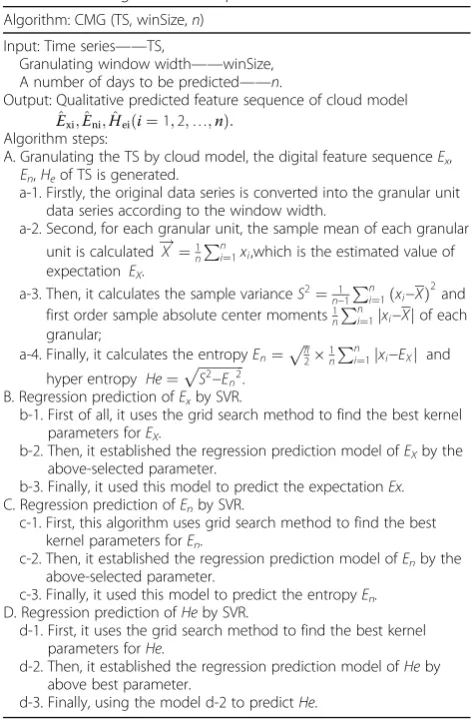
drop, the uncertainty of cloud drop is smaller. Therefore, the exception Ex was selected as the prediction values of the target. Specifically, the proposed algorithm based on cloud model granulation (CMG) is described in Table3:
3 Results and discussion
3.1 Forecast results of air quality index
As mentioned above, the time series data of APs and AQIs show non-linearly characteristics over time, which are also missing, inconsistent, heterogeneous, and uncertain. It in-dicates that the approaches of dealing with uncertainty might perform better in air quality forecasting. In this study, it used three approaches: the support vector regres-sion (SVR) (Vapnik, 1995), Non-linear autoregressive neural network(NAR), and the proposed SVR algorithm based on cloud model granulation, to predict the target AQIt + 1. In our experiments, the set of training dataOtrain (used in the procedure of learning) contained the 2016 an-nual data (366 data points) and the set of testing data Otest from 2017.1.1~ 2017.1.7 (7 data points). In order to avoid overlearning, it used the 5-fold cross-validation to select the optimum values of the approaches’parameters.
In this study, all the SVR approaches use the ε -insensitive loss function in the regularized risk func-tional that ensures optimum generalization performance. In addition, The radial basis function kernel (RBF) was used in LIBSVM toolbox [25]. In the experiments, the epsilon in loss function of epsilon-SVR is set to 0.01. The grid search method is used to find the optimum kernel parameter with penalty parameter C= [−10, 10] and kernel parameterg= [−10, 10].
NAR employed here is one kind of dynamic neural network, which can use to solve a non-linear time series problem with the non-linear autoregressive neural net-work model. The structures and parameters of the NARs were also found by a grid search method for the follow-ing values: (1) the maximum number of neurons in the hidden layer ranged was set from 10 to 100; (2) the delay days were set to {3, 7, 15, 90} in order to the fairness of comparative experiments.
The CMG algorithm refers to the presented SVR ap-proach based on cloud model concept extraction. Like above SVR approach, the CMG uses ε-SVR for the pre-diction of exception Ex, entropy En, and hyper excep-tion He. The RBF kernel was used in sequential minimal optimization (SMOreg) for training SVR with the kernel parameter g= [−10, 10] and penalty param-eter C= [−10, 10]. According to the season effect of air quality forecasting and the physical meaning of gran-ules, the experiments tested different values of the win-dow width winSize={3, 7, 15, 30, 90};
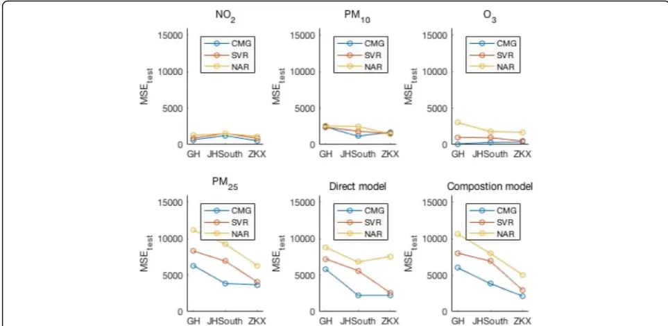
Figure 4 presented the MSEtest of AQI prediction on both composition models and the direct models. The re-sults indicate that the CMG algorithm trained on the direct model gets the lowest MSEtestof AQI. In contrast, the highest MSEtest error for the direct model was ob-tained using NAR. In the composition model, the lowest MSEtest was also the achieved by the CMG algorithm. This observation means that, when compared with other popular artificial intelligence algorithms like SVR and NAR, the proposed CMG is able to cope with the lower amount of data in the process of learning and testing.
To further study the performance of CMG, MSEtest ex-periments on all determinative pollutant was performed. It is obvious that the CMG algorithm performed best on the four determinative pollutants for all localities, except for the PM10 prediction in ZKX locality. While the Nar performed worse in most cases. The results for SVR are slightly inferior to CMG in most cases. It can be found that the high error of PM25 seems to generate a high MSEtest in the process of AQF. It occurred despite the low errors on NO2, PM10, and O3. The former is almost four times that of the latter in all localities. The MSEtest for NO2 was, for all methods, almost the same in the case of GH, JHS, and ZKX, respectively. For the ZKX locality, the MSEtest of SVR and CMG was always lower Table 3CMG algorithm description
Algorithm: CMG (TS, winSize,n)
Input: Time series——TS,
Granulating window width——winSize, A number of days to be predicted——n.
Output: Qualitative predicted feature sequence of cloud model
^
Exi;Eni^ ;Hei^ ði¼1;2;…;nÞ: Algorithm steps:
A. Granulating the TS by cloud model, the digital feature sequenceEx,
En,Heof TS is generated.
a-1. Firstly, the original data series is converted into the granular unit data series according to the window width.
a-2. Second, for each granular unit, the sample mean of each granular unit is calculated! ¼X 1
n
Pn
i¼1xi,which is the estimated value of expectation EX.
a-3. Then, it calculates the sample varianceS2¼ 1 n−1
Pn i¼1ðxi−XÞ
2 and first order sample absolute center moments1
nPni¼1jxi−Xjof each
B. Regression prediction ofExby SVR.
b-1. First of all, it uses the grid search method to find the best kernel parameters forEX.
b-2. Then, it established the regression prediction model ofEXby the
above-selected parameter.
b-3. Finally, it used this model to predict the expectationEx. C. Regression prediction ofEnby SVR.
c-1. First, this algorithm uses grid search method to find the best kernel parameters forEn.
c-2. Then, it established the regression prediction model ofEnby the
above-selected parameter.
c-3. Finally, it used this model to predict the entropyEn.
D. Regression prediction ofHeby SVR.
d-1. First, it uses the grid search method to find the best kernel parameters forHe.
d-2. Then, it established the regression prediction model ofHeby above best parameter.
with the similar values on both IAQI prediction and AQI forecasting. This occurred despite the various between other methods on different localities. To sum up, these re-sults advised that the prediction performance was related to the algorithms and the datasets. But, CMG algorithm performed best for both IAQI prediction and AQI models compared with other two algorithms.
3.2 Forecast results of air quality index class
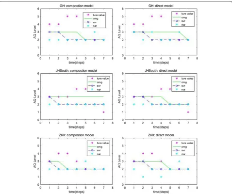
In human life, the AQI class is the most desired, not the AQI. The prediction ability of the AQI class is one of the most interesting topics for AQI prediction model. There-fore, the above prediction values of AQI were transformed into corresponding AQI class. As shown in Fig.5, it com-pared the predictive classification results of the compos-ition models and direct models at three localities. It is not difficult to find that patterns of the test data were only presented in the 1–5 AQI class. Finally, the test accuracy of AQI class was calculated to evaluate the classification performance. Table 4showed the percentage of correctly classified patterns of various prediction models. It shows that the direct model based on CMG for ZKX performed best up to 71.43%. The performance of CMG and SVR run better in most experiments.
As can be seen from Fig.2, the vast majority of air qual-ity classes can be divided into four AQI classes in three lo-calities. In addition, the analysis of the classification results in Fig.5shows that the proposed CMG approaches
for measuring misclassification were mainly divided into the adjacent class, i.e., from (3→2 or 3→4), from (3→2 or 3→4), from 1→2. Only in very few cases are divided into interval classes.
3.3 Analysis and discussion
After the data exploration, the results show that the pro-posed CMG approach can give better performance in both IAQI and AQI forecasting. The exploration of in-put data provides an understanding of the data compos-ition of raw data. The results of the variability (mean and standard deviation) of IAQIs and AQIs indicate that the overall air quality in three localities is generally simi-lar, but the features are locality specific. Specifically, in all localities, the percentage of the second and third clas-ses are significantly higher than other clasclas-ses, and the fifth classes have the fewest number of days. But it is worth noting that the proportion of the first class is sig-nificantly lower than the fourth class in GH, which is a contract to that in JHS and ZK. Most importantly, it is found that PM25 and O3 accounted for most of the major determinative pollutants. In this study, it proposed a new algorithm based on cloud model granulation. This paper compared the performance of three approaches (nar, svr, and CMG) on both composition model and dir-ect model in three regions.
The high importance of cloud model granulation in the prediction models gives a strategy for solving Fig. 4MSEtestfor AQI prediction. The first subgraph shows the MSEtestof three algorithms (CMG, SVR, NAR) for NO2prediction. The second
subgraph shows the MSEtestof three algorithms (CMG, SVR, NAR) for PM10prediction. The third subgraph shows the MSEtestof three algorithms
(CMG, SVR, NAR) for O3 prediction. The fourth subgraph shows the MSEtestof three algorithms (CMG, SVR, NAR) for PM25prediction. The fifth
subgraph shows the MSEtestof three algorithms (CMG, SVR, NAR) for AQI prediction on direct model. The sixth subgraph shows the MSEtestof
problems at a higher thinking Level. It uses only three numerical features (expectation, entropy, hyper) to de-scribe the randomness, fuzziness, and their relevance of time series data. This model enables complex data to form information granules with semantic descriptions and mine complex data in the new feature space, which
is in line with human thinking and background know-ledge of air quality forecasting in the real world.
In order to achieve more accurate forecasting and fair, several important artificial intelligence algorithms in AQF are compared on composition models and direct models. As expected, the designed algorithm is overall Fig. 5Prediction of AQI class. The first subgraph shows three methods of predicting the AQL class by the composition model at the GH location. The second subgraph shows the results of three algorithms (CMG, SVR, NAR) for AQI class prediction by direct model at GH locality. The third subgraph shows the results of three algorithms (CMG, SVR, NAR) for AQI class prediction by composition model at JHS locality. The fourth subgraph shows the results of three algorithms (CMG, SVR, NAR) for AQI class prediction by direct model at JHS locality. The fifth subgraph shows the results of three algorithms (CMG, SVR, NAR) for AQI class prediction by composition model at ZKX locality. The sixth subgraph shows the results of three algorithms (CMG, SVR, NAR) for AQI class prediction by direct model at ZKX locality
Table 4Prediction accuracy of AQI class
CMG SVR NAR
Com-model Dir-model Com-model Dir-model Com-model Dir-model
GH 42.86% 14.29% 42.86 42.86% 28.57% 28.57%
JHSouth 42.86% 42.86% 14.29% 28.57% 0 0
optimal due to its ability to process uncertain informa-tion and remarkable generalizainforma-tion, especially in O3 pre-diction. In addition, the SVR approach performs better, which corroborates the findings of a great deal of the previous work in this field of AQF [1,17]. In the case of the AQI class’ prediction, similar to AQIs forecasting, the proposed algorithm and SVR showed the promising result. The instances of misclassification are basically placed into neighboring classes.
3.4 Limitations and future work
In general, a number of important improvements of this study need to be considered. First of all, the experiments use free public data, which includes only the IAQI of APs and AQI. If more chemical and meteorological conditions information obtained, the study may get more accurate prediction results. Second, it replaced the missing data with the mean or most. It may lead to biased results. The
ε-insensitive SVR with semi-supervised learning approach may use unlabeled data with missing output values. Therefore, it may be effectively used for further study. In the future, we will employ multiple output SVR for con-sidering the error between the true value and prediction value. In addition, because classification performance was strongly influenced by class size balance, it may use the optimized classifier to solve this problem in the case of the imbalanced dataset. Last but not least, the structural model of cloud model granulation can not only enable to give a rational approach for the value prediction of IAQIs or AQIs but can also be used to estimate target’s confi-dence interval. It hopes that the prediction range of true value can be calculated according to the given member-ship range, which can be used in other data with uncertain.
4 Conclusions
This paper proposed one novel algorithm based on cloud model granulation for air quality forecasting, whose data is non-linear, uncertain, and heterogeneous. After iterative granulation of original time series, the proposed algorithm extracted the conceptual features of cloud model for each new granule. Then, the cloud model feature is used as the operating space for problem solving. The CMG algorithm gives the solution to the problem by inferring the eigenvalues of future granules. The experimental results show that this algorithm can not only simplify the modeling process of uncertain time series in the form of knowledge abstraction, but also has good predictive performance in IAQI and AQI.
Compared with previous literature, this is the first at-tempt to predict AQIs by cloud model granulation. This method not only considers the fuzziness and random-ness of the problem as a whole, but also transforms the problems in the original data space to the feature space
and from feature space to concept space. Finally, the so-lution to the original problem is accomplished by con-tinuous data reduction, without concern for the original data distribution characteristics. This algorithm does not only design for the time series of air quality forecasting. Its aim is to provide a new solution based on state space transformation and cloud model granulation for time series with uncertainty. There is a large research field that researchers and engineers must make more effort around data mining, machine learning, and artificial intelligence with uncertainty that these will brings light to big data. It is hoped that this will inspire readers to continue to explore cloud models to deal with the uncertainties in the real world.
Abbreviation
ML:Machine Learning; APs: Air pollutants; AQF: Air quality forecasting; AQI: Air Quality Index; GH: Ganghua of Qingshan District; JHS: South area of Jianghan District; LIBSVM: A Library for Support Vector Machines;
MEP: Ministry of Environmental Protection; NARNNs: Non-linear
Autoregressive Neural Networks; NNs: Neural networks; SC: Soft computing; SVR: Support vector regression; ZKX: New area of Zhuankou locality
Acknowledgements
The authors would like to thank Prof. Shuliang Wang at Beijing Institute of Technology, Beijing, China, for the help of collecting the data of this work.
Funding
This work is supported by National Natural Science Foundation of China (Grant No. 61763002), Guangxi Natural Science Foundation (Grant No. 2015GXNSFBA139249), and the Joint special of Shandong Natural Science Foundation of the China Republic under Grant No: (ZR2017LF020).
Availability of data and materials
All the experiment data is obtained from Wuhan Municipal Environmental Protection Bureau, which can be freely accessed and download on its official website.
Authors’contributions
YL and YS proposed the main idea of CMG together. YL is the main writer of this paper, wrote the code of CMG algorithm, and completed the
experiments. YS analyzed the result and gave the feasible improvement plans. LZ provided the implementation solution for implementing key problems related to concept extraction by cloud model. HL simulated the transition from AQI to AQL. All authors read and approved the final manuscript.
Competing interests
The authors declare that they have no competing interests.
Publisher’s Note
Springer Nature remains neutral with regard to jurisdictional claims in published maps and institutional affiliations.
Author details
1Computer School, Wuhan University, Wuhan, China.2School of Computer
and Electronics and Information, Guangxi University, Nanning, China.3School of Information, Qilu University of Technology (Shandong Academy of Sciences), Jinan, China.4School of Resource and Environmental Science,
Received: 16 February 2018 Accepted: 18 April 2018
References
1. P Hajek, Predicting common air quality index—The case of czech microregions. Aerosol Air Qual. Res.15(2), 544–555 (2015)
2. B Bukoski, EM Taylor, Air quality forecasting. Air Qual. Manage.87, 563–586 (2014)
3. G Zhou, J Xu, Y Xie, L Chang, W Gao, Y Gu, J Zhou, Numerical air quality forecasting over eastern China: An operational application of WRF-Chem. Atmos. Environ.153, 94–108 (2017)
4. M Pascal, M Corso, O Chanel, C Declercq, C Badaloni, G Cesaroni, S Henschel, K Meister, D Haluza, P Martin-Olmedo, Assessing the public health impacts of urban air pollution in 25 European cities: Results of the Aphekom project. Sci. Total Environ.449, 390–400 (2013)
5. P Hájek, V Olej, Ozone prediction on the basis of neural networks, support vector regression and methods with uncertainty. Ecol. inform.12, 31–42 (2012) 6. N Haizum, A Rahman, MH Lee, MT Latif, Artificial neural networks and fuzzy
time series forecasting: An application to air quality. Qual. Quant.49, 2633 (2015)
7. M El-Harbawi, Air quality modelling, simulation, and computational methods: A review. Environ. Rev.21, 149–179 (2013)
8. I Kyriakidis, K Karatzas, G Papadourakis, A Ware, J Kukkonen, Investigation and forecasting of the common air quality index in Thessaloniki, Greece. Artif. Intell. Appl. Innov.382(2), 390–400 (2012)
9. A Kumar, P Goyal, Forecasting of air quality index in Delhi using neural network based on principal component analysis. Pure Appl. Geophys.170, 711–722 (2013)
10. Y Zhang, M Bocquet, V Mallet, C Seigneur, A Baklanov, Real-time air quality forecasting, part I: History, techniques, and current status. Atmos. Environ.
60, 632–655 (2012)
11. A Kumar, P Goyal, Air quality prediction of PM10 through analytical dispersion model for Delhi. Aerosol Air Qual. Res.14(5), 1487–1499 (2014) 12. A Donnelly, B Misstear, B Broderick, Real time air quality forecasting using integrated parametric and non-parametric regression techniques. Atmos. Environ.103, 53–65 (2015)
13. J Westerlund, JP Urbain, J Bonilla, Application of air quality combination forecasting to Bogota. Atmos. Environ.89, 22–28 (2014)
14. A-L Dutot, J Rynkiewicz, FE Steiner, J Rude, A 24-h forecast of ozone peaks and exceedance levels using neural classifiers and weather predictions. Environ. Model Softw.22, 1261–1269 (2007)
15. W Tamas, G Notton, C Paoli, M-L Nivet, C Voyant, Hybridization of air quality forecasting models using machine learning and clustering: An original approach to detect pollutant peaks. Aerosol Air Qual. Res.16, 405–416 (2015)
16. M Awad, R Khanna, Support vector regression. Neural Inf. Process. Lett. Rev.
11(10), 203–224 (2007)
17. K-P Lin, P-F Pai, S-L Yang, Forecasting concentrations of air pollutants by logarithm support vector regression with immune algorithms. Appl. Math. Comput.217, 5318–5327 (2011)
18. D Domańska, M Wojtylak, Application of fuzzy time series models for forecasting pollution concentrations. Expert Syst. Appl.39, 7673–7679 (2012) 19. JT Connor, RD Martin, LE Atlas, Recurrent neural networks and robust time
series prediction. IEEE Trans. Neural Netw.5, 240–254 (1994)
20. EK Cairncross, J John, M Zunckel, A novel air pollution index based on the relative risk of daily mortality associated with short-term exposure to common air pollutants. Atmos. Environ.41, 8442–8454 (2007) 21. S van den Elshout, K Léger, H Heich, CAQI common air quality
index—Update with PM 2.5 and sensitivity analysis. Sci. Total Environ.488, 461–468 (2014)
22. Library, W. P. (2013). Ministry of Environmental Protection of the people's Republic of China.
23. G Asadollahfardi, SH Aria, M Mehdinejad, The prediction of atmospheric concentrations of toluene using artificial neural network methods in Tehran. Adv. Environ. Res.4, 219–231 (2015)
24. A Sadiq, A El Fazziki, J Ouarzazi, M Sadgal, Towards an agent based traffic regulation and recommendation system for the on-road air quality control. SpringerPlus5, 1604 (2016)
25. C-C Chang, C-J Lin, LIBSVM: A library for support vector machines. ACM Trans. Intell. Syst. Technol. (TIST)2, 27 (2011)
26. D Li, C Liu, W Gan, A new cognitive model: Cloud model. Int. J. Intell. Syst.
24, 357–375 (2009)
27. C Xu, G Wang, Q Zhang, A new multi-step backward cloud transformation algorithm based on normal cloud model. Fundamenta Informaticae133(1), 55–85 (2014)