Global dynamics of a general diffusive HBV infection model with capsids and adaptive immune response

R E S E A R C H

Open Access

Global dynamics of a general diffusive

HBV infection model with capsids

and adaptive immune response

A.M. Elaiw

_{and A.D. Al Agha}

*_{Correspondence:} [email protected] 1_{Department of Mathematics,}

Faculty of Science, King Abdulaziz University, Jeddah, Saudi Arabia

Abstract

This paper studies the global dynamics of a general diffusive hepatitis B virus (HBV) infection model. The model includes both enveloped viruses and DNA containing capsids. Two immune responses are recruited to attack the virus and infected hepatocytes. These are the cytotoxic T-lymphocytes (CTL) which kill the infected liver cells, and B cells which send antibodies to attack the virus. The non-negativity and boundedness of the solutions are discussed. The existence of spatially homogeneous equilibrium points is examined. The global stability of all possible equilibrium points is proved by choosing suitable Lyapunov functionals. Some numerical simulations are performed to enhance the theoretical results and present the behavior of solutions in space and time.

Keywords: HBV infection; Capsids; Adaptive immune response; Diffusion; Global stability; Lyapunov function

1 Introduction

Liver plays a central role in many functions of the body. Hepatitis B virus (HBV) is a hep-adnavirus that infects hepatocytes (liver cells) and leads to acute or chronic infections [1]. The chronic hepatitis B can develop into cirrhosis and hepatocellular carcinoma, which may lead to death [2,3]. According to the global hepatitis report from the World Health Organization [2], chronic HBV caused about 884,400 deaths in 2015 and approximately 257 million people are infected with the virus. During the life cycle of the virus, HBV DNA containing capsid has important functions in virus formation and replication [3–5]. The capsid can be enveloped and released from the infected cell as virus particles. The adaptive immune system has a crucial role in fighting the virus. It sends cytotoxic T cells (known as cytotoxic T-lymphocytes (CTL)) to kill the infected liver cells, and B cells that generate antibodies to attack the virus [1,6].

Mathematical models have been used to understand the HBV dynamics and test the hypotheses that are difficult to apply in laboratory. The basic virus dynamics model was proposed by Nowak and Bangham in 1996 [7]. However, in this model and many other ex-tended models (see, for example, [8–19]) it was assumed that cells and viruses are equally distributed in the domain. Also, their ability to move was ignored despite the fact that

their motion may have a critical role in biological systems [20]. After that, many works have started to incorporate spatial diffusion into the biological models in order to make them more realistic. For example, Wang and Wang [21] assumed that the movement of the HBV follows the Fickian diffusion [22] and studied the following model:

⎧ ⎪ ⎪ ⎨ ⎪ ⎪ ⎩

∂U(x,t)

∂t =λ–dU(x,t) –γU(x,t)V(x,t),

∂I(x,t)

∂t =γU(x,t)V(x,t) –αI(x,t),

∂V(x,t)

∂t =dVV(x,t) +kI(x,t) –mV(x,t),

(1)

whereU(x,t),I(x,t), andV(x,t) represent the densities of uninfected hepatocytes, infected hepatocytes, and free HBV at positionxand timet, respectively. The target cells are pro-duced at rateλ, die at ratedU, and are converted into infected cells at rateγUV. The infected cells die at rateαI, while the viruses die at ratemV. The viruses diffuse with a dif-fusion coefficientdVand are generated from infected cells at ratekI. In the diffusion term,

V=∂_∂2_xV2 is the Laplacian operator. Xu and Ma [23] studied a diffusive HBV model with time delay and saturation infection rate. Shaoli et al. [24] investigated an HBV infection model with virus diffusion and nonlinear infection rate. Zhang and Xu [25] considered a delayed HBV model with Beddington–DeAngelis infection rate and diffusion. Miao et al. [6] developed an infection model consisting of five partial differential equations, time delays, and adaptive immunity. In a very recent work, Bellomo and Tao [26] studied a vi-ral infection model with diffusion induced by chemotaxis dynamics. More recently, many works have added an explicit equation for HBV nucleocapsids to some HBV infection models. For example, Geng et al. [27] considered the mobility of capsids and viruses and applied the nonstandard finite difference (NSFD) scheme to discretize a continuous HBV infection model with capsids. Their work was an extension to the work of Manna and Chakrabarty [28]. Guo et al. [29] studied an HBV infection model which contains three time delays, capsids, general incidence rate, and allows the movement of viruses by diffu-sion. Manna [30] investigated the role of the CTL immune response in a reaction-diffusion model of HBV with capsids. Notably, none of the aforementioned models considered both capsids and adaptive immune response.

equilibrium points. In Sect.5, we perform some numerical simulations to support the obtained theoretical results. The conclusion is stated in Sect.6.

2 A diffusive HBV dynamics model with capsids and adaptive immune response

Motivated by the work of [6,13,30,31], we study the following general HBV infection model with capsids and two forms of adaptive immune response:

⎧ ⎪ ⎪ ⎪ ⎪ ⎪ ⎪ ⎪ ⎪ ⎪ ⎪ ⎪ ⎨ ⎪ ⎪ ⎪ ⎪ ⎪ ⎪ ⎪ ⎪ ⎪ ⎪ ⎪ ⎩

∂U(x,t)

∂t =Θ(U(x,t)) –Π(U(x,t),V(x,t)),

∂I(x,t)

∂t =Π(U(x,t),V(x,t)) –αΦ1(I(x,t)) –δΦ1(I(x,t))Φ4(Z(x,t)),

∂C(x,t)

∂t =dCC(x,t) +bΦ1(I(x,t)) – (α+β)Φ2(C(x,t)),

∂V(x,t)

∂t =dVV(x,t) +βΦ2(C(x,t)) –mΦ3(V(x,t)) –rΦ3(V(x,t))Φ5(W(x,t)),

∂Z(x,t)

∂t =pΦ1(I(x,t))Φ4(Z(x,t)) –σ Φ4(Z(x,t)),

∂W(x,t)

∂t =qΦ3(V(x,t))Φ5(W(x,t)) –μΦ5(W(x,t)),

(2)

where U(x,t),I(x,t),C(x,t),V(x,t),Z(x,t), andW(x,t) stand for the densities of unin-fected hepatocytes, inunin-fected hepatocytes, HBV nucleocapsids, HBV particles, CTLs, and B cells at locationxand timet, respectively. The functionΘ(U) is the intrinsic growth rate including both the production and death rates of hepatocytes. The functionΠ(U,V) gives the rate at which the uninfected hepatocytes become infected. The infected cells are killed by CTLs at rateδΦ1(I)Φ4(Z) and die at rateαΦ1(I). The coefficientdCis the

diffu-sion coefficient of capsids. The virus capsids are produced from infected liver cells at rate

bΦ1(I) and used to form enveloped virus particles at rateβΦ2(C). The capsids and viruses

die at ratesαΦ2(C) andmΦ3(V), respectively. Viruses are neutralized by antibodies at rate

rΦ3(V)Φ5(W). CTLs are stimulated in response to antigens at ratepΦ1(I)Φ4(Z), while B

cells are stimulated to produce antibodies at rateqΦ3(V)Φ5(W). The CTL and B immune

cells die at ratesσ Φ4(Z) andμΦ5(W), respectively.

For model (2), we consider the following initial conditions:

U(x, 0) =ψ1(x)≥0, I(x, 0) =ψ2(x)≥0, C(x, 0) =ψ3(x)≥0,

V(x, 0) =ψ4(x)≥0, Z(x, 0) =ψ5(x)≥0, W(x, 0) =ψ6(x)≥0, x∈ ¯Ω,

(3)

and homogeneous Neumann boundary conditions

∂C

∂n = 0,

∂V

∂n = 0, fort> 0,x∈∂Ω. (4)

The functionsψi(i= 1, . . . , 6) are Hölder continuous inΩ¯. The domainΩis connected

and bounded with a smooth boundary∂Ω. In addition,_∂∂_nrepresents differentiation in the direction of the outward normal to the boundary∂Ω. The Neumann boundary conditions imply that no virus particles or capsids pass through or exit the boundary.

The general functionsΘ,Π, andΦi(i= 1, . . . , 5) are continuous, differentiable and meet

the following requirements: [Q1] (i) Θ(U) < 0for allU> 0,

(iii) there are two parametersκ1> 0andκ2> 0such thatΘ(U)≤κ1–κ2Ufor all

This section discusses some fundamental properties of the solutions of model (2)–(4) to be biologically valid. These properties include the existence, positivity, and boundedness of the solutions. Also, we show that model (2) has five equilibrium points under some threshold conditions.

Theorem 1 Assume that requirements[Q1]–[Q3]are met,then there exists a unique so-lution of model (2)defined on[0, +∞)for any initial data satisfying(3).Moreover, this solution is nonnegative and bounded for t≥0.

Proof LetX=BUC(Ω¯,R6_{) be the set of all bounded and uniformly continuous functions}

It follows from [25,34,35] that, for anyψ∈X+, system (2)–(4) has a unique non-negative

mild solution on [0,Tl), where [0,Tl) is the maximal existence time interval.

Now, we show the boundedness of the solutions. Take

B1(x,t) =U(x,t) +I(x,t) + δ

pZ(x,t).

Using requirements [Q1] and [Q3] with model (2) leads to

∂B1(x,t) ∂t =Θ

U(x,t)–αΦ1

I(x,t)–σ δ

p Φ4

Z(x,t)

≤κ1–κ2U(x,t) –αρ1I(x,t) – σ δρ4

p Z(x,t)

≤κ1–s1B1(x,t),

wheres1=min{κ2,αρ1,σρ4}. Thus,

B1(x,t)≤max

κ1

s1

,max

x∈ ¯Ω

ψ1(x) +ψ2(x) + δ

pψ5(x)

:=ζ1,

which implies thatU(x,t),I(x,t), andZ(x,t) are bounded. Moreover, from the bounded-ness ofI(x,t), the third equation of (2) and [Q3], we get

⎧ ⎪ ⎪ ⎨ ⎪ ⎪ ⎩

∂C

∂t –dCC(x,t)≤bΦ1(ζ1) – (α+β)ρ2C(x,t),

∂C

∂n= 0,

C(x, 0) =ψ3(x)≥0.

LetC(t) be a solution to the following ordinary differential equation:

⎧ ⎨ ⎩

dC

dt =bΦ1(ζ1) – (α+β)ρ2C,

C(0) =max_{x∈ ¯Ω}ψ3(x).

Hence, it follows thatC(t)≤max{bΦ1(ζ1)

(α+β)ρ2,maxx∈ ¯Ωψ3(x)}. According to the comparison principle [36],C(x,t)≤C(t). So,

C(x,t)≤max

bΦ1(ζ1)

(α+β)ρ2,maxx∈ ¯Ω

ψ3(x) :=ζ2.

Finally, we prove the boundedness ofV(x,t) andW(x,t). Using the boundedness ofC(x,t) and from model (2)–(4), we find thatV(x,t) satisfies the following system:

⎧ ⎪ ⎪ ⎨ ⎪ ⎪ ⎩

∂V

∂t –dVV(x,t)≤βΦ2(ζ2) –mΦ3(V(x,t)) –rΦ3(V(x,t))Φ5(W(x,t)),

∂V

∂n = 0,

LetV(t) be a solution to the following system: ⎧

⎨ ⎩

dV

dt =βΦ2(ζ2) –mΦ3(V) –rΦ3(V)Φ5(W(x,t)),

V(0) =max_{x∈ ¯Ω}ψ4(x).

The comparison principle givesV(x,t)≤V(t). Denote

B2(x,t) =V(t) +

r qW(x,t),

then using [Q3], we obtain

∂B2(x,t)

∂t =βΦ2(ζ2) –mΦ3(V) –

μr q Φ5

W(x,t)

≤βΦ2(ζ2) –mρ3V– μρ5r

q W(x,t)

≤βΦ2(ζ2) –s2B2(x,t),

wheres2=min{mρ3,μρ5}. This implies thatV(t)≤max{βΦ_s2₂(ζ2),maxx∈ ¯Ω{ψ4(x) +r_qψ6(x)}}.

Then we get

V(x,t)≤max

βΦ2(ζ2)

s2

,max

x∈ ¯Ω

ψ4(x) +

r qψ6(x)

:=ζ3,

W(x,t)≤q

rζ3.

Thus, the above discussion assures the boundedness of U(x,t), I(x,t), C(x,t), V(x,t),

Z(x,t), andW(x,t) onΩ¯×[0,Tl). Then the boundedness of the solutions onΩ¯×[0, +∞)

follows from the standard theory for semi-linear parabolic systems [37] whereTl= +∞.

Theorem 2 Suppose that all requirements[Q1]–[Q4]are met,then there are five threshold parameters which determine the existence of five possible equilibrium points of model(2)

as follows:

(i) the model has an infection-free equilibriumM0ifR0≤1,

(ii) the model has an immune-free equilibriumM1ifR1≤1 <R0andR2≤1 <R0,

(iii) the model has an infection equilibriumM2with only antibody immune response if

R1> 1andR3≤1,

(iv) the model has an infection equilibriumM3with only CTL immune response ifR2> 1

and R1

R3 ≤1,

(v) the model has an infection equilibriumM4with both antibody and CTL immune

responses ifR1>R3> 1.

Proof Any equilibrium pointM= (U,I,C,V,Z,W) of system (2) satisfies the following equilibrium conditions:

Θ(U) –Π(U,V) = 0, (5)

bΦ1(I) – (α+β)Φ2(C) = 0, (7)

βΦ2(C) –mΦ3(V) –rΦ3(V)Φ5(W) = 0, (8)

pΦ1(I)Φ4(Z) –σ Φ4(Z) = 0, (9)

qΦ3(V)Φ5(W) –μΦ5(W) = 0. (10)

From Eq. (9) we get (pΦ1(I) –σ)Φ4(Z) = 0, which gives two possible options

Φ1(I) =σ

p or Φ4(Z) = 0. (11)

Also, from Eq. (10) we have (qΦ3(V) –μ)Φ5(W) = 0, which gives two possible options

Φ3(V) = μ

q or Φ5(W) = 0. (12)

Then, according to (11) and (12), there are four cases:

Case 1.IfΦ4(Z) = 0 andΦ5(W) = 0, then by [Q3] we getZ= 0 andW= 0.

Thus, equilibrium conditions (5)–(10) are reduced to

Θ(U) –Π(U,V) = 0, (13)

Π(U,V) –αΦ1(I) = 0, (14)

bΦ1(I) – (α+β)Φ2(C) = 0, (15)

βΦ2(C) –mΦ3(V) = 0. (16)

From Eqs. (13)–(16) we obtain the following relations:

Π(U,V) =Θ(U), (17)

and

Φ1(I) =

1

αΘ(U), Φ2(C) =

b

α(α+β)Θ(U), Φ3(V) =

bβ

mα(α+β)Θ(U). (18)

We can conclude from [Q3] thatΦ_i–1(i= 1, . . . , 5) exist, strictly increasing andΦ_i–1(0) = 0. Then we define

Γ1(U) =Φ₁–1

1

αΘ(U)

, Γ2(U) =Φ₂–1

b

α(α+β)Θ(U)

,

Γ3(U) =Φ3–1

bβ

mα(α+β)Θ(U)

.

(19)

Hence, it follows from (18) and (19) that

I=Γ1(U), C=Γ2(U), V=Γ3(U). (20)

We note from [Q1] thatΓ1(U0) =Γ2(U0) =Γ3(U0) = 0. Equations (17)–(20) give

ΠU,Γ3(U)

–mα(α+β)

bβ Φ3

Γ3(U)

Using Eq. (20) along with requirements [Q1]–[Q3], we can see that Eq. (21) admits a so-lutionU=U0, and this gives the disease-free equilibriumM0= (U0, 0, 0, 0, 0, 0).

Denote

χ1(U) =Π

U,Γ3(U)

–mα(α+β)

bβ Φ3

Γ3(U)

= 0. (22)

Based on [Q1]–[Q3], we find

χ1(0) = –

mα(α+β)

bβ Φ3

Γ3(0)

< 0,

χ1(U0) = 0.

Now, in order to have a root in the interval (0,U0), we need to show thatχ1(U0) < 0.

χ₁(U0) =

∂Π(U0, 0) ∂U +

∂Π(U0, 0) ∂V Γ

3(U0) –

mα(α+β)

bβ Φ

3(0)Γ3(U0).

Since∂Π(U0,0)

∂U = 0 by [Q2], then from (18) and (20) we get

χ₁(U0) =

mα(α+β)

bβ Φ

3(0)Γ3(U0)

bβ

mα(α+β)Φ₃(0)

∂Π(U0, 0) ∂V – 1

=Θ(U0)

bβ

mα(α+β)Φ₃(0)

∂Π(U0, 0) ∂V – 1

=Θ(U0)(R0– 1),

whereR0is the basic reproduction number and is given by

R0=

bβ

mα(α+β)Φ₃(0)

∂Π(U0, 0) ∂V .

AsΘ(U0) < 0 by [Q1], thenχ1(U0) < 0 ifR0> 1. Therefore, whenR0> 1, there exists a

rootU1∈(0,U0) such thatχ1(U1) = 0. From Eq. (20) and requirements [Q1]–[Q3], the

corresponding components are

I1=Γ1(U1) > 0, C1=Γ2(U1) > 0, V1=Γ3(U1) > 0.

Thus, the immune-free equilibrium M1 = (U1,I1,C1,V1, 0, 0) exists if R0> 1. In other

words, the threshold conditionR0> 1 is needed for the infection pointM1to exist in the

absence of immune responses.

Case 2.IfΦ3(V) =μ_q andΦ4(Z) = 0, then the third requirement [Q3] implies that

V2=Φ3–1

μ

q

> 0 and Z2= 0.

SubstitutingV=V2in (5) givesΘ(U) –Π(U,V2) = 0.

Let

Then, with the aid of [Q1] and [Q2] we get

χ2(0) =Θ(0) > 0,

χ2(U0) = –Π(U0,V2) < 0,

χ₂(U) =Θ(U) –∂Π(U,V2)

∂U < 0.

Accordingly, there exists a unique root U2∈(0,U0) of (23) such thatχ2(U2) = 0. From

Eq. (20) and [Q1]–[Q3], we get

I2=Γ1(U2) > 0, C2=Γ2(U2) > 0.

Finally, from Eqs. (5)–(8) we obtain

W2=Φ5–1

bβ

rα(α+β)

Π(U2,V2) Φ3(V2)

–m

r

=Φ₅–1

m

r

bβ

mα(α+β)

Π(U2,V2) Φ3(V2)

– 1

=Φ₅–1

m

r(R1– 1)

> 0 ifR1> 1,

whereR1is defined as

R1=

bβ

mα(α+β)

Π(U2,V2) Φ3(V2)

.

R1is the threshold number needed for activating the antibody immune response against

viruses. Hence, the infection equilibrium with only antibody immune defense M2 =

(U2,I2,C2,V2, 0,W2) exists ifR1> 1.

Using [Q2]–[Q4], we can note that

R1≤

bβ

mα(α+β)Vlim→0+

Π(U2,V) Φ3(V)

= bβ

mα(α+β)Φ₃(0)

∂Π(U2, 0) ∂V

< bβ

mα(α+β)Φ₃(0)

∂Π(U0, 0) ∂V =R0.

Case 3.IfΦ1(I) =σ_p andΦ5(W) = 0, we get

I3=Φ1–1

σ

p

> 0 and W3= 0.

Then Eqs. (7) and (8) give

C3=Φ2–1

bσ

p(α+β)

> 0 and V3=Φ3–1

bβσ

mp(α+β)

> 0.

Denote

χ3(U) =Θ(U) –Π(U,V3) = 0.

According to requirements [Q1] and [Q2],χ3(U) is strictly decreasing and

χ3(0) =Θ(0) > 0,

χ3(U0) = –Π(U0,V3) < 0.

Thus,χ3(U) has a unique rootU3∈(0,U0) such thatχ3(U3) = 0. From Eqs. (5)–(8), we

have

Z3=Φ4–1

bβ

mδ(α+β)

Π(U3,V3) Φ3(V3)

–α

δ

=Φ₄–1

α δ

bβ

mα(α+β)

Π(U3,V3) Φ3(V3)

– 1

=Φ₄–1

α δ(R2– 1)

> 0 ifR2> 1,

whereR2is given by

R2=

bβ

mα(α+β)

Π(U3,V3) Φ3(V3)

.

Here,R2represents the activation number for CTL immune defense. Thus, the infection

equilibrium without antibody immune responseM3= (U3,I3,C3,V3,Z3, 0) exists ifR2> 1.

According to [Q2]–[Q4], it is easy to note that

R2≤

bβ

mα(α+β)Vlim→0+

Π(U3,V) Φ3(V)

= bβ

mα(α+β)Φ₃(0)

∂Π(U3, 0) ∂V

< bβ

mα(α+β)Φ₃(0)

∂Π(U0, 0) ∂V =R0.

Case 4.IfΦ1(I) =σ_p andΦ3(V) =μ_q, then we get

I4=Φ1–1

σ

p

> 0 and V4=Φ3–1

μ

q

> 0.

Then Eq. (7) gives

C4=Φ2–1

bσ

p(α+β)

> 0.

ReplaceV byV4in Eq. (5) and define

Using [Q1] and [Q2], we can see thatχ4(U) is strictly decreasing,χ4(0) > 0 andχ4(U0) < 0.

Thus, there exists a unique rootU4∈(0,U0) such thatχ4(U4) = 0.

Eq. (6) is used to obtain

Z4=Φ4–1

α δ

Π(U4,V4) αΦ1(I4)

– 1

=Φ₄–1

α δ

pμ ασq

Π(U4,V4) Φ3(V4)

– 1

=Φ₄–1

α δ(R3– 1)

> 0 ifR3> 1,

whereR3is a threshold parameter defined by

R3=

pμ ασq

Π(U4,V4) Φ3(V4)

.

Finally, Eq. (8) is used to get

W4=Φ5–1

bβσq pμr(α+β)–

m r

.

SinceV2=V4, thenU2=U4. Hence, we have

W4=Φ5–1

m

r

R1

R3

– 1

> 0 ifR1>R3,

where R1

R3 is given by

R1

R3

= bβσq

mpμ(α+β).

Thus, the infection equilibrium with CTL and antibody immune defenseM4= (U4,I4,C4,

V4,Z4,W4) exists ifR1>R3> 1. That is, the two immune responses work together to fight

the virus whenR1>R3> 1.

4 Global stability

In this section we study the global stability of the five equilibrium pointsM0,M1,M2,M3,

andM4of system (2) by using the Lyapunov method.

Theorem 3 Let requirements[Q1]–[Q4] be satisfied, then the disease-free equilibrium M0= (U0, 0, 0, 0, 0, 0)is globally asymptotically stable if R0≤1.

Proof Define

Λ0(t) =

Ω

Λ0x(x,t) dx,

where

Λ0x(x,t) =U–U0–

U U0

lim

V→0+

Π(U0,V) Π(ϕ,V) dϕ+I+

α

bC+

α(α+β)

bβ V+

δ

pZ+

rα(α+β)

–δσ

From the divergence theorem and (4), we have

In addition, we deduce from [Q1] and [Q2] that

Accordingly, Eq. (24) is reduced to

dΛ0

It follows from system (2) thatI= 0 andC= 0. Accordingly, the largest invariant set in {(U,I,C,V,Z,W) :dΛ0

dt = 0}is the singleton{M0}. Thus, by LaSalle’s invariance principle

[38], the infection-free equilibriumM0is globally asymptotically stable whenR0≤1.

Lemma 1 Suppose that R0> 1and[Q1]–[Q4]are valid,then

sgn(U2–U1) =sgn(V1–V2) =sgn(R1– 1).

Proof From [Q1], [Q2], and [Q4], we can conclude the following relations:

Consequently, from (26)–(28) we havesgn(U1–U2) =sgn(U2–U1), which is a

contradic-tion. This implies that

sgn(U2–U1) =sgn(V1–V2).

Moreover, using (17) and (18) with the definition ofR1gives

R1– 1 =

bβ

mα(α+β)

Π(U2,V2) Φ3(V2)

– bβ

mα(α+β)

Π(U1,V1) Φ3(V1)

= bβ

mα(α+β)

Π(U2,V2) Φ3(V2)

–Π(U1,V1)

Φ3(V1)

= bβ

mα(α+β)

1

Φ3(V2)

Π(U2,V2) –Π(U1,V2)

+Π(U1,V2)

Φ3(V2)

–Π(U1,V1)

Φ3(V1)

.

Thus, from (27)–(29) we have

sgn(V1–V2) =sgn(R1– 1).

Lemma 2 If R0> 1and[Q1]–[Q4]hold,then

sgn(U3–U1) =sgn(V1–V3) =sgn(I1–I3) =sgn(R2– 1).

Proof From [Q1], [Q2], and [Q4], we have

(U1–U3)

Θ(U3) –Θ(U1)

> 0, (30)

(U3–U1)

Π(U3,V3) –Π(U1,V3)

> 0, (31)

(V3–V1)

Π(U1,V3) –Π(U1,V1)

> 0, (32)

(V1–V3)

Π(U1,V3) Φ3(V3)

–Π(U1,V1)

Φ3(V1)

> 0 (33)

forU1,U3,V1,V3> 0. From the equilibrium conditions ofM1andM3, we get

Φ1(I1) =

m(α+β)

bβ Φ3(V1),

Φ1(I3) =

m(α+β)

bβ Φ3(V3),

which implies that sgn(V1–V3) =sgn(I1–I3). Using (30)–(33) and following the same

strategies used for proving Lemma1, we can show that

sgn(U3–U1) =sgn(V1–V3)

and

Theorem 4 Assume that requirements[Q1]–[Q4]are met,then the infection equilibrium

without immune responses M1= (U1,I1,C1,V1, 0, 0)is globally asymptotically stable if R1≤

1 <R0and R2≤1 <R0.

Proof Introduce a Lyapunov functional

At the equilibrium pointM1, we have

Thus, (34) can be rewritten as follows:

+

We can deduce from the divergence theorem and Neumann boundary conditions that

0 =

Rearranging and using [Q3], we get

Using Lemma1and2and [Q3], we have

Φ1(I1) –Φ1(I3)≤0 ifR2≤1,

Φ3(V1) –Φ3(V2)≤0 ifR1≤1.

Using the relation between geometrical and arithmetical means, we have

5≤Π(U1,V1)

The above arguments imply thatdΛ1

dt ≤0 ifR1≤1 andR2≤1. It is easy to check that

principle [38] assures its global asymptotic stability.

Theorem 5 The infection equilibrium with only antibody immune response M2= (U2,I2,

C2,V2, 0,W2)is globally asymptotically stable if R1> 1,R3≤1and whenever [Q1]–[Q4]

are satisfied.

Proof Consider a Lyapunov functional

+δ

From the equilibrium conditions ofM2, we observe

Θ(U2) =Π(U2,V2),

Using the equilibrium pointsM2andM4, we have

SinceV2=V4, then by Theorem2we haveU2=U4. This implies that

Theorem 6 Suppose that[Q1]–[Q4]are valid,then the infection equilibrium with only CTL immune response M3= (U3,I3,C3,V3,Z3, 0) is globally asymptotically stable when

R2> 1andR_R1₃ ≤1.

Proof Take a Lyapunov functional as

+1

By using the equilibrium conditions atM3

Θ(U3) =Π(U3,V3),

and collecting terms of (42), we have

+r(α+β)(α+δΦ4(Z3))

Using the equilibrium pointsM3andM4, we have

Φ3(V3) =

The other terms are less than or equal to zero for the same reasons given in (38) and (39), therefore dΛ3

dt = 0}. By LaSalle’s invariance principle [38], the equilibrium point

M3is defined and globally asymptotically stable ifR2> 1 andR_R1₃ ≤1. Theorem 7 Assume that requirements[Q1]–[Q4]are met,then the infection equilibrium with CTL and antibody immune responses M4= (U4,I4,C4,V4,Z4,W4)is globally

asymp-totically stable when R1>R3> 1.

Proof Define a Lyapunov functional

Then we obtain

By using the equilibrium conditions atM4

Θ(U4) =Π(U4,V4),

and collecting terms of (43), we have

Table 1 List of parameters of model (44)

Parameter Value Source Parameter Value Source

λ 10 cells mm–3day–1 References [39,40] r 0.9 mm3_cell–1_day–1 _Assumed

m 8 day–1 Assumed ς1 Varied Assumed

–Φ2(C)Φ3(V4)

M4is globally asymptotically stable by LaSalle’s invariance principle [38], where the point

exists ifR1>R3> 1.

5 Numerical simulations

Our goal in this section is to carry out some numerical simulations which exhibit the global stability of all equilibrium points of the model. We consider the following special case of model (2):

where the infection rateΠ(U,V) is the Beddington–DeAngelis functional response [25,

42,43]. It is straightforward to check that all requirements [Q1]–[Q4] are satisfied. We assume the following initial conditions:

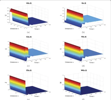
Figure 1The numerical simulations of system (44)–(46) whenR0≤1. The infection-free equilibriumM0is

globally asymptotically stable. The sub-figures show the spatiotemporal behaviors of (a) uninfected hepatocytes, (b) infected hepatocytes, (c) capsids, (d) viruses, (e) CTLs, and (f) B cells

C(x, 0) = 10 capsids mm–3, V(x, 0) = 2 virions mm–3, (45)

Z(x, 0) = 1.5 cells mm–3, W(x, 0) = 1 cells mm–3, x∈[0, 1],

and homogeneous Neumann boundary conditions

∂C

∂n = 0,

∂V

∂n = 0, fort∈[0, 500],x= 0, 1. (46)

The initial values are arbitrarily chosen as the global stability of the equilibrium points guarantees the convergence regardless of the selected initial conditions. The threshold parametersR0,R1,R2, andR3are given by

R0=

bβγ λ

mα(α+β)(d+ς1λ),

R1=

bβqγU2

mα(α+β)(q+qς1U2+ς2μ)

,

R2=

bβpγU3

mpα(α+β)(1 +ς1U3) +ας2bβσ

,

R3=

pμγU4 ασ(q+qς1U4+ς2μ)

Figure 2The numerical simulations of system (44)–(46) whenR1≤1 <R0andR2≤1 <R0. The immune-free

equilibriumM1is globally asymptotically stable. The sub-figures show the spatiotemporal behaviors of

(a) uninfected hepatocytes, (b) infected hepatocytes, (c) capsids, (d) viruses, (e) CTLs, and (f) B cells

where

U2=U4= 1 2ς1dq

ς1λq–ς2dμ–γ μ–dq+

(ς1λq–ς2dμ–γ μ–dq)2+ 4ς1dq(ς2λμ+λq)

,

U3=

mp(α+β)(ς1λ–d) –bβσ(ς2d+γ) 2ς1dmp(α+β)

+

(mp(α+β)(ς1λ–d) –bβσ(ς2d+γ))2+ 4ς1dmp(α+β)(αλmp+βλmp+bβς2λσ)

2ς1dmp(α+β) .

For the numerical simulations of system (44)–(46), the values ofγ,p,μ, andς1are changed

as they have the most important effects on the global stability of equilibrium points. The values of all other parameters are fixed in Table1. We have chosen the parameters of the model to perform the numerical simulations. This is because of the difficulty of getting real data from HBV infected patients; however, if one has real data, then the parameters of the model can be estimated and the validity of the model can be established.

The results can be divided into the following categories:

(i) Whenγ = 0.9mm3_virus–1_day–1_{,p= 0.2mm}3_cell–1_day–1_{,μ= 0.1day}–1_and ς1= 1mm3cell–1, then we getR0= 0.0524 < 1. In this case, the solutions of system

Figure 3The numerical simulations of system (44)–(46) whenR1> 1 andR3≤1. The infection equilibrium

M2is globally asymptotically stable. The sub-figures show the spatiotemporal behaviors of (a) uninfected

hepatocytes, (b) infected hepatocytes, (c) capsids, (d) viruses, (e) CTLs, and (f) B cells

Actually, this result supports Theorem3and represents the case when the liver cells are completely uninfected and the infection is finished out.

(ii) Whenγ = 0.5mm3_virus–1_day–1_{,p= 0.01mm}3_cell–1_day–1_{,μ= 1.5day}–1_and ς1= 0.02mm3cell–1, then we find0.5482 =R1< 1 <R0= 1.3889and

0.7569 =R2< 1 <R0= 1.3889. For this set of parameters and according to

Theorem4, the solutions of system (44) converge to the immune-free equilibrium

M1= (162.3944, 13.9603, 2.7921, 0.4886, 0, 0)as shown in Fig.2. The number of

uninfected hepatocytes drops sharply when the HBV infection is chronic and the immune responses are not active.

(iii) We takeγ = 0.5mm3_virus–1_day–1_{,p= 0.01mm}3_cell–1_day–1_{,μ= 0.5day}–1_and ς1= 0.02mm3cell–1. These values giveR0= 1.3889 > 1,R1= 1.2023 > 1, and

R3= 0.5725 < 1. In agreement with the result of Theorem5, the infection

equilibriumM2= (313.1212, 11.4516, 2.2903, 0.3334, 0, 1.7987)is globally

Figure 4The numerical simulations of system (44)–(46) whenR2> 1 andRR1₃≤1. The infection equilibrium M3is globally asymptotically stable. The sub-figures show the spatiotemporal behaviors of (a) uninfected

hepatocytes, (b) infected hepatocytes, (c) capsids, (d) viruses, (e) CTLs, and (f) B cells

(iv) Ifγ= 0.5mm3_virus–1_day–1

,p= 0.07mm3_cell–1

day–1,μ= 0.5day–1and

ς1= 0.01mm3cell–1, then we obtainR0= 2.6515 > 1,R2= 2.4515 > 1, and

R1

R3 = 0.3 < 1. For this choice of parameter values, the solutions of system (44) converge to the infection equilibrium

M3= (579.4083, 2.775, 0.5546, 0.097, 0.8672, 0), which supports Theorem6. The

results are shown in Fig.4. In this situation, CTL immune response works alone to kill the infected cells which are the source of the virus.

(v) Whenγ = 0.7mm3_virus–1_day–1_{,p= 0.15mm}3_cell–1_day–1_{,μ= 0.06day}–1_and ς1= 0.01mm3cell–1, then we getR0= 3.7121 > 1,R3= 3.0757 > 1, R_R1₃ = 1.1667 > 1.

In agreement with Theorem7, we can see from Fig.5that the equilibrium

M4= (753.4535, 1.3449, 0.2708, 0.0406, 1.2688, 1.5117)is globally asymptotically

stable. Here, CTL and antibody immune responses work in parallel to kill the infected hepatocytes and attack the HBV, respectively. As a result, the number of healthy liver cells increases while the numbers of infected cells, capsids, and viruses decrease.

6 Conclusion

Figure 5The numerical simulations of system (44)–(46) whenR3> 1 andR1>R3> 1. The equilibrium with

two immune responsesM4is globally asymptotically stable. The sub-figures show the spatiotemporal

behaviors of (a) uninfected hepatocytes, (b) infected hepatocytes, (c) capsids, (d) viruses, (e) CTLs, and (f) B cells

model has five equilibrium points which are given by the disease-free equilibriumM0,

the immune-free equilibriumM1, the infection equilibrium with only antibody immune

responseM2, the infection point with only CTL immune responseM3, and the

equilib-rium with both types of adaptive immunityM4. The conditions for existence and global

stability of these equilibrium points have produced four threshold parametersR0,R1,R2,

andR3. The equilibrium pointM0is globally asymptotically stable ifR0≤1, which

indi-cates that the liver cells are totally healthy and there is no infection. The equilibriumM1

exists and is globally asymptotically stable ifR1≤1 <R0 andR2≤1 <R0, and it reflects

the situation when the immune responses have not been activated yet to counter the in-fection. The infection equilibriumM2exists and is globally asymptotically stable ifR1> 1

andR3≤1, where only B lymphocytes work to defeat the virus. On the other hand,M3

exists and is globally asymptotically stable equilibrium point ifR2> 1 and R_R1₃ ≤1. In this

case, only CTLs try to clear the infection by killing the infected hepatocytes. Finally, B and T immune cells work together to eliminate HBV infection at the equilibriumM4that

exists and is globally asymptotically stable ifR1>R3> 1. The provided numerical

It is commonly observed that in viral infection processes, time delay is inevitable (see, e.g., [8–11,44–47]). Extending model (2) to include the effect of treatments and time de-lays will give a deeper insight into HBV infection. Another extension of model (2) is to incorporate stochastic interactions (see [48]). We leave these points as future works.

Acknowledgements

This project funded by the Deanship of Scientific Research (DSR), King Abdulaziz University, Jeddah, under grant No. (DF-005-130-1441). The authors, therefore, gratefully acknowledge DSR technical and financial support.

Funding

Not applicable.

Availability of data and materials

Not applicable.

Competing interests

The authors declare that they have no competing interests.

Authors’ contributions

All authors contributed equally to the writing of this paper. All authors read and approved the final manuscript.

Publisher’s Note

Springer Nature remains neutral with regard to jurisdictional claims in published maps and institutional affiliations.

Received: 26 April 2019 Accepted: 3 December 2019

References

1. Nowak, M.A., May, R.M.: Virus Dynamics: Mathematical Principles of Immunology and Virology. Oxford University Press, Oxford (2000)

2. World Health Organization: Global Hepatitis Report 2017. World Health Organization, Geneva (2017). License: CCBY-NC-SA 3.0 IGO

3. Pairan, A., Bruss, V.: Functional surfaces of the hepatitis B virus capsid. J. Virol.83, 11616–11623 (2009) 4. Bruss, V.: Envelopment of the hepatitis B virus nucleocapsid. Virus Res.106, 199–209 (2004)

5. Grimm, D., Thimme, R., Blum, H.E.: HBV life cycle and novel drug targets. Hepatol. Int.5(2), 644–653 (2011)

6. Miao, H., Teng, Z., Abdurahman, X., Li, Z.: Global stability of a diffusive and delayed virus infection model with general incidence function and adaptive immune response. Comput. Appl. Math.37(3), 3780–3805 (2018)

7. Nowak, M.A., Bangham, C.R.M.: Population dynamics of immune responses to persistent viruses. Science272, 74–79 (1996)

8. Huang, G., Takeuchi, Y., Ma, W.: Lyapunov functionals for delay differential equations model of viral infections. SIAM J. Appl. Math.70(7), 2693–2708 (2010)

9. Elaiw, A.M., Elnahary, E.Kh., Raezah, A.A.: Effect of cellular reservoirs and delays on the global dynamics of HIV. Adv. Differ. Equ.2018, Article ID 85 (2018)

10. Hobiny, A.D., Elaiw, A.M., Almatrafi, A.: Stability of delayed pathogen dynamics models with latency and two routes of infection. Adv. Differ. Equ.2018, Article ID 276 (2018)

11. Elaiw, A.M., Raezah, A.A., Azoz, S.A.: Stability of delayed HIV dynamics models with two latent reservoirs and immune impairment. Adv. Differ. Equ.2018, Article ID 414 (2018)

12. Hattaf, K., Yousfi, N.: A generalized virus dynamics model with cell-to-cell transmission and cure rate. Adv. Differ. Equ. 2016, Article ID 174 (2016)

13. Elaiw, A.M., AlShamrani, N.H.: Stability of an adaptive immunity pathogen dynamics model with latency and multiple delays. Math. Methods Appl. Sci.41(16), 6645–6672 (2018)

14. Shu, H., Wang, L., Watmough, J.: Global stability of a nonlinear viral infection model with infinitely distributed intracellular delays and CTL immune responses. SIAM J. Appl. Math.73(3), 1280–1302 (2013)

15. Carvalho, A.R.M., Pinto, C.M.A., Baleanu, D.: HIV/HCV coinfection model: a fractional-order perspective for the effect of the HIV viral load. Adv. Differ. Equ.2018, Article ID 2 (2018)

16. Elaiw, A.M., Almuallem, N.A.: Global properties of delayed-HIV dynamics models with differential drug efficacy in cocirculating target cells. Appl. Math. Comput.265, 1067–1089 (2015)

17. Elaiw, A.M., AlShamrani, N.H.: Stability of a general adaptive immunity virus dynamics model with multi-stages of infected cells and two routes of infection. Math. Methods Appl. Sci. (2019).https://doi.org/10.1002/mma.5923

18. Elaiw, A.M., Alshaikh, M.A.: Stability analysis of a general discrete-time pathogen infection model with humoral immunity. J. Differ. Equ. Appl. (2019).https://doi.org/10.1080/10236198.2019.1662411

19. Huang, G., Ma, W., Takeuchi, Y.: Global properties for virus dynamics model with Beddington–DeAngelis functional response. Appl. Math. Lett.22(11), 1690–1693 (2009)

20. Britton, N.F.: Essential Mathematical Biology. Springer, London (2003)

21. Wang, K., Wang, W.: Propagation of HBV with spatial dependence. Math. Biosci.210, 78–95 (2007)

22. Gourley, S.A., So, J.W.H.: Dynamics of a food-limited population model incorporating nonlocal delays on a finite domain. J. Math. Biol.44, 49–78 (2002)

24. Shaoli, W., Xinlong, F., Yinnian, H.: Global asymptotical properties for a diffused HBV infection model with CTL immune response and nonlinear incidence. Acta Math. Sci.31B(5), 1959–1967 (2011)

25. Zhang, Y., Xu, Z.: Dynamics of a diffusive HBV model with delayed Beddington–DeAngelis response. Nonlinear Anal., Real World Appl.15, 118–139 (2014)

26. Bellomo, N., Tao, Y.: Stabilization in a chemotaxis model for virus infection. Discrete Contin. Dyn. Syst., Ser. S13(2), 105–117 (2020)

27. Geng, Y., Xu, J., Hou, J.: Discretization and dynamic consistency of a delayed and diffusive viral infection model. Appl. Math. Comput.316, 282–295 (2018)

28. Manna, K., Chakrabarty, S.P.: Global stability and a non-standard finite difference scheme for a diffusion driven HBV model with capsids. J. Differ. Equ. Appl.21(10), 918–933 (2015)

29. Guo, T., Liu, H., Xu, C., Yan, F.: Global stability of a diffusive and delayed HBV infection model with HBV DNA-containing capsids and general incidence rate. Discrete Contin. Dyn. Syst., Ser. B23, 4223–4242 (2018)

30. Manna, K.: Dynamics of a delayed diffusive HBV infection model with capsids and CTL immune response. Int. J. Appl. Comput. Math.4, Article ID 116 (2018).https://doi.org/10.1007/s40819-018-0552-4

31. Danane, J., Allali, K.: Mathematical analysis and treatment for a delayed hepatitis B viral infection model with the adaptive immune response and DNA-containing capsids. High-Throughput7, Article ID 35 (2018).

https://doi.org/10.3390/ht7040035

32. Xu, J., Geng, Y.: Threshold dynamics of a delayed virus infection model with cellular immunity and general nonlinear incidence. Math. Methods Appl. Sci.42(3), 892–906 (2018)

33. Min, L., Su, Y., Kuang, Y.: Mathematical analysis of a basic virus infection model with application to HBV infection. Rocky Mt. J. Math.38(5), 1573–1585 (2008)

34. Xu, Z., Xu, Y.: Stability of a CD4+T cell viral infection model with diffusion. Int. J. Biomath.11(5), Article ID 1850071 (2018)

35. Smith, H.L.: Monotone Dynamical Systems: An Introduction to the Theory of Competitive and Cooperative Systems. Am. Math. Soc., Providence (1995)

36. Protter, M.H., Weinberger, H.F.: Maximum Principles in Differential Equations. Prentice Hall, Englewood Cliffs (1967) 37. Henry, D.: Geometric Theory of Semilinear Parabolic Equations. Springer, New York (1993)

38. Hale, J.K., Verduyn Lunel, S.M.: Introduction to Functional Differential Equations. Springer, New York (1993) 39. Perelson, A., Kirschner, D., De Boer, R.: Dynamics of HIV infection of CD4+ T cells. Math. Biosci.114(1), 81–125 (1993) 40. Culshaw, R., Ruan, S., Spiteri, R.: Optimal HIV treatment by maximising immune response. J. Math. Biol.48(5), 545–562

(2004)

41. Pawelek, K., Liu, S., Pahlevani, F., Rong, L.: A model of HIV-1 infection with two time delays: mathematical analysis and comparison with patient data. Math. Biosci.235(1), 98–109 (2012)

42. Beddington, J.R.: Mutual interference between parasites or predators and its effect on searching efficiency. J. Anim. Ecol.44, 331–340 (1975)

43. DeAngelis, D.L., Goldstein, R.A., O’Neill, R.V.: A model for tropic interaction. Ecology56, 881–892 (1975)

44. Elaiw, A.M., Elnahary, E.Kh.: Analysis of general humoral immunity HIV dynamics model with HAART and distributed delays. Mathematics7, Article ID 157 (2019)

45. Elaiw, A.M., Almatrafi, A., Hobiny, A.D., Hattaf, K.: Global properties of a general latent pathogen dynamics model with delayed pathogenic and cellular infections. Discrete Dyn. Nat. Soc.2019, Article ID 9585497 (2019)

46. Elaiw, A.M., Raezah, A.A.: Stability of general virus dynamics models with both cellular and viral infections and delays. Math. Methods Appl. Sci.40(16), 5863–5880 (2017)

47. Elaiw, A.M., Alshehaiween, S.F., Hobiny, A.D.: Global properties of delay-distributed HIV dynamics model including impairment of B-cell functions. Mathematics7, Article ID 837 (2019)