Processing the Bouguer anomaly map of Biga and the surrounding area by the
cellular neural network: application to the southwestern Marmara region
Davut Aydogan
Istanbul University, Engineering Faculty, Department of Geophysics, 34310, Avcilar, Istanbul, Turkey
(Received May 25, 2006; Revised December 22, 2006; Accepted December 25, 2006; Online published May 7, 2007)
An image processing technique called the cellular neural network (CNN) approach is used in this study to locate geological features giving rise to gravity anomalies such as faults or the boundary of two geologic zones. CNN is a stochastic image processing technique based on template optimization using the neighborhood relationships of cells. These cells can be characterized by a functional block diagram that is typical of neural network theory. The functionality of CNN is described in its entirety by a number of small matrices (A,BandI) called the cloning template. CNN can also be considered to be a nonlinear convolution of these matrices. This template describes the strength of the nearest neighbor interconnections in the network. The recurrent perceptron learning algorithm (RPLA) is used in optimization of cloning template. The CNN and standard Canny algorithms were first tested on two sets of synthetic gravity data with the aim of checking the reliability of the proposed approach. The CNN method was compared with classical derivative techniques by applying the cross-correlation method (CC) to the same anomaly map as this latter approach can detect some features that are difficult to identify on the Bouguer anomaly maps. This approach was then applied to the Bouguer anomaly map of Biga and its surrounding area, in Turkey. Structural features in the area between Bandırma, Biga, Yenice and Gonen in the southwest Marmara region are investigated by applying the CNN and CC to the Bouguer anomaly map. Faults identified by these algorithms are generally in accordance with previously mapped surface faults. These examples show that the geologic boundaries can be detected from Bouguer anomaly maps using the cloning template approach. A visual evaluation of the outputs of the CNN and CC approaches is carried out, and the results are compared with each other. This approach provides quantitative solutions based on just a few assumptions, which makes the method more powerful than the classical methods.
Key words: CNN, derivative method, cross-correlation, Canny algorithm, cloning template, gravity anomaly, geological features, southwestern Marmara region, Turkey.
1.
Introduction
One of the most common problems encountered in geo-physical studies is how to determine the subsurface geolog-ical features, namely faults or the boundary of two geologic zones at various depths, as it difficult to establish the geo-logical boundaries hidden beneath surface materials. Grav-ity is an effective geophysical method by which to identify these, and numerous techniques exist in the field of geo-physics for analyzing gravity anomalies produced by faults or the boundary of two geologic zones. In this context, boundary analyses of gravity or magnetic anomalies are car-ried out using various combinations of directional derivative (gradient) techniques. Edge detection algorithms are used for analyzing potential sets of field data, such as gravity and magnetic maps, in order to detect main geological bodies, subtle geological features, geological structures and align-ments (Boschetti, 2005). Since the early 1970s, a variety of automatic or semiautomatic methods, all of which are based on the use of the horizontal or vertical gradient of potential field anomalies, have been developed as efficient tools for
Copyright cThe Society of Geomagnetism and Earth, Planetary and Space Sci-ences (SGEPSS); The Seismological Society of Japan; The Volcanological Society of Japan; The Geodetic Society of Japan; The Japanese Society for Planetary Sci-ences; TERRAPUB.
the determination of geometric parameters, such as loca-tions of boundaries and the depths of the causative sources. Since potential field data correspond to the superposition of effects from all causative sources, the determination of ge-ologic boundaries usually suffers from nearby source inter-ference that produces false edges. Most of the images need to be enhanced before an edge detection scheme can be ap-plied successfully. Image enhancement is a general term describing the process of manipulating the data in an image to emphasize the features of interest. Of the many methods that exist to evaluate edge detectors, the Canny algorithms (1986) were the first to provide analytic expressions for the criteria that have to be optimized in edge detection.
Geologists and geophysicists are interested in linear anomalies in gravity and magnetic maps that may corre-spond to subsurface faults, a boundary of two geologic zones and other structural features. The Radon transform is a useful method for analyzing lineaments in a two-dimensional (2-D) map, and Sykes and Das (2000) have used this approach transform to enhance linear features in geophysical maps. Boschetti (2005) proposed a number of edge detection algorithms based on gravity gradient. In ad-dition, several edge detection algorithms can be found in earlier publications, all of which are based on image
which they used to analyze gravity and magnetic anomalies. In this technique, various orders of horizontal derivatives are summed, and the vertical derivative is then taken; the location of maxima is used to outline the source boundaries. Zenget al.(1994) proposed a technique which is based on cross-correlation (CC) between the theoretical anomaly due to a vertical step and the second vertical derivative of the Bouguer anomaly to locate minor faults that may be diffi-cult to identify based only on the Bouguer anomaly map. In this approach, faults are located from the closed maxima or minima on the CC map. Blakely and Simpson (1986) improved the boundary analysis technique, which detects buried geological structures based on the horizontal deriva-tive of gravity data.
The cellular neural network (CNN) approach can also be used for edge detection, data enhancement and the separa-tion of potential field maps. The most popular applicasepara-tion of CNN has been image processing, essentially because of its analog feature and sparse connections, all of which are conductive to real time processing. The dynamics of the CNN approach are described by a system of nonlinear or-dinary differential equations and by an associated compu-tation energy function that is minimized during the com-putation process. A two-dimensional CNN can be consid-ered to be a two-dimensional filter and has been applied for noise removal, shape extraction and edge detection. In the present study, CNN is used in the edge detection of geolog-ical structures. We show that this approach is a useful tool for detecting deep faults, even in presence of shallower near surface features.
Aydogan et al.(2005) recently introduced the CNN al-gorithm, providing implicitly the expressions necessary to apply the method to the analysis of gravity data. For those interested readers who are not familiar with neural network data analysis techniques, this article is barely comprehensi-ble. In this article, I therefore explicitly provide the details of this method so that any reader will be able to follow the method easily and use it for routine applications. In addi-tion to the numerical examples provided by Aydoganet al.
(2005), I also introduce more complex numerical models to illustrate the power of the CNN algorithm. One of the major outcomes of this paper is its contribution to the seismotec-tonics of the southwestern Marmara sea region where we identify a hidden fault that is not present at the active fault maps of Turkey.
2.
Cellular Neural Network Approach
The CNN model was introduced by Chua and Yang (1988a, b) and consists of a recurrent nonlinear network in which neurons are locally connected and the dynamics are identical for each node. These neurons are commonly called cells. The connection with the cells outside ther -neighborhood is enabled by the propagation effects of the network dynamics. The dynamics of a CNN is described
an output. Any one cell is connected only to its neigh-boring cells. The cell located in the position (i,j) of a
where the size of the neighborhoodr is a positive integer number.
The state equation for cellCi jis defined as follows:
∂xi j(t) bias of cellCi j, respectively. The state and output vary in time, while the input is static (time independent). Matrices
Ai j,kl, which are the feedback template coefficients (deriva-tive coefficients), andBi j,kl, which are the control template coefficients, are connected from cellCkl toCi j. The matri-ces A(·), B(·)andI are known collectively as the cloning template. The feedback control template represents the cou-pling coefficients of the cells, and this completely defines the behavior of the network with a given input and initial condition.
The output equation is described by the following piece-wise linear equation:
yi j(t)= f(xi j(t))=.5xi j(t)+1−xi j(t)−1, (3)
where f can be any convenient non-linear function, such as the signum, sigmoid or step function.
A significant feature of CNN is that it has two indepen-dent input capabilities: the generic input and the initial state of the cells. These are normally bounded by
ui j(t)≤1 and xi j(0)≤1. (4)
Similarly, if|f(.)| ≤1 thenyi j(t)≤1.
As can be seen, the input is represented by the intensity values of the pixels that are stored in the matrixu, while the initial state values are stored in the matrixx.
The functionality of the CNN array can be controlled by the cloning template (A, B andI), where A andB are
(2r+1)×(2r+1)real matrices andI is a scalar number in two-dimensional CNNs. In many applications, A and B are space-invariant.
Fig. 1. A two-dimensional CNN defined on a squared grid, a) Thei j-th cell of the array is colored by black, b) The neighborhood function
Nr(c)forr=1, c)r=2 (neighbor cells are black).
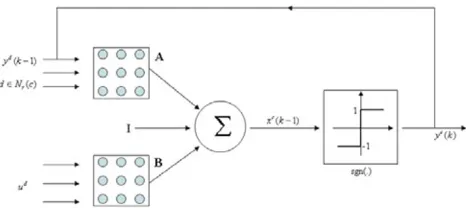
Fig. 2. Block scheme of the DT-CNN cell. xi j,ui j,yi j andIi j are the state, input and output and bias of cellCi j, respectively.
wherecxdenotes the row andcydenotes the column. Each cell connects directly with the set of cells that are within a certain distancer ofc. This set is ther-neighborhood that is defined forr≥0 by:
Nr(c)=d ∈ Z2maxdy−cy,|dx−cx|
≤r. (5)
Forr=1 andr=2, ther-neighborhood is shown in Fig. 1. At the discrete timek, the statexcof a cellcdepends on the time-independent inputudapplied to its neighboring cellsd and the time-variant outputs yd(k). The cell state equation is given by:
xc(k)=
d∈Nr(c)
Ayd(k)+
d∈Nr(c)
Bud+I. (6)
Consequently, the output of cell c at time stepk > 0 is obtained by threshold state ofcat timek−1:
yc(k)=sgn(xc(k−1))
=
+1 f or xc(k−1)≥0
−1 f or xc(k−1)≺0 . (7)
In the case of non-zero feedback coefficients, the output fork=0 needs to be specified. As in differential equations where the solution depends on the initial conditions, the initial outputyc(0)is of crucial importance to the behavior of the system. In the case when all feedback coefficients are zero, the initial output does not influence the final output of the system. The output of the system remains constant after the first time step. The block diagram of a DT-CNN is demonstrated in Fig. 2.
3.
Template Design for the CNN
The design of templates A,BandI are necessary if the CNN approach is to be used for gray scale image process-ing. A learning procedure can be applied to estimate these
Fig. 3. Learning algorithm scheme.
templates, which determine the desired CNN behavior. All global learning methods are based on minimizing an error function (ε)—that is a function defined in terms of the de-sired network output and the actual network output. In this study, the recurrent perceptron learning algorithm (RPLA) is used. The form of the template is as follows:
A=
a2 a1 a2
a1 a0 a1
a2 a1 a2
, B=
b2 b1 b2
b1 b0 b1
b2 b1 b2
, I. (8)
For stability templateA,Bshould be symmetrical anda0 must be greater than zero for edge detection. This template,
w, can be defined as a vector:
w=[a0 a1 a2 b0 b1 b2 I]. (9)
whereai denotes the feedback coefficients,bi denotes the control coefficients andI is the cell bias or threshold.
The error function of all cells is shown as:
ε[w]= c
i,j
(yic,j−d c
i,j)2, (10)
whereyis the actual output anddis the desired output. A learning procedure scheme is shown in Fig. 3. A 2-D CNN can be viewed as a 2-D filter and can be applied for noise removal, shape extraction and edge detection.
4.
Application to Synthetic Data
4.1 Multiple sources (model 1)
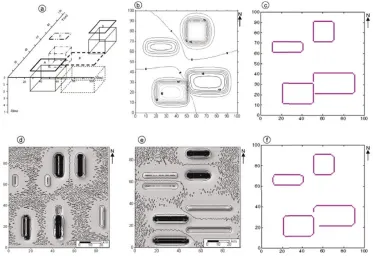
In this section, synthetic models are used to check the reliability of the proposed approach. Some practical re-sults are presented and briefly discussed to demonstrate the success of the proposed algorithm. The synthetic gravity anomaly map shown in Fig. 4(b) was produced by using finite rectangular vertical prisms located at various depths. The prisms B and C are deeper than the prisms A and D (Fig. 4(a)). In the present study, it is assumed that 1 pixel corresponds to 1 km. The model is 101×101 pixels wide.
Fig. 4. Synthetic example: (a) Schematic outlines of model 1, (b) synthetic anomaly map (contour interval is 2 mGal), (c) edge map from CNN, (d) gray-shaded relief of cross-correlation map in the E-W direction, (e) gray-shaded relief of cross-correlation map in the N-S direction, (f) edge map obtained by standard Canny algorithm. Cross-correlation maps are illuminated from the NW.
is used to optimize the cloning template. Forr = 1, this optimal template is determined to be:
A=
0 0 0
0 2 0
0 0 0
,
B=
−.51 −.51 −.51 −.51 5.8 −.51 −.51 −.51 −.51
, I = −2.6.
(11)
During the learning procedure, in feedback matrix, only the a0 coefficient is found to be greater than zero, while in the control matrix, all coefficients are −0.51, except
for b0, which is 5.8. In this case, the control coefficients
(bi) are qualitatively the same as the coefficients of the derivative method. Finally, the bias value I is estimated to be−2.6. This is necessary for network stability and edge detection. This cloning template describes the strength of the nearest-neighbor interconnections in the network. The proposed approach with the cloning template given in Eq. (11) is applied on the anomaly map of model 1, and CNN output is demonstrated in Fig. 4(c). CNN can be seen here to delineate the edges of the prisms quite well. To compare the proposed approach with classical derivative techniques, the CC method is applied onto the same gravity anomaly map. This method is based on CC between the synthetic anomaly due to a vertical step and the second vertical derivative of the gravity anomaly. The CC for a finite length of the second vertical derivative of the synthetic anomaly due to a step gt(x), (x = −n, . . . ,0, . . . ,n), and the second vertical derivative of the observed anomaly
go(x),(x =1,2, . . . ,m), can be expressed as
rgogt(x)= n
x=−n
go(x+x)gt(x) (12)
wherex=n+1,n+2, . . . ,m−nandn<m.
The CC maps in the E-W and N-S directions are ob-tained by Eq. (12) as shown in Figs. 4(d), (e). The edges of the prisms are located from the closed maxima or minima on these maps calculated for two perpendicular directions. Since some small closed extrema may be produced by high-frequency noise in the second vertical derivative map, only the closed extrema with a clear elongation direction are cho-sen. Although the outputs derived from the CC analysis are somewhat noisy (Figs. 4(d), (e)), the CNN method yields quite distinct prism borders (Fig. 4(c)).
The edges of the prisms are determined using the stan-dard Canny algorithm (Fig. 4(f)) as well. The results of the Canny and CNN algorithms are similar in the case of simple models.
In summary, it can be stated that CNN is the more pow-erful tool for detecting the border of a vertical prism.
4.2 Multiple sources (model 2)
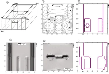
Fig. 5. Synthetic example: (a) Schematic outlines of model 2, (b) synthetic anomaly map (contour interval is 10 mGal), (c) edge map obtained from CNN, (d) gray-shaded relief of cross-correlation map in the E-W direction, (e) gray-shaded relief of cross-correlation map in the N-S direction, (f) edge map obtained by standard Canny algorithm. Cross-correlation maps are illuminated from the NW.
edges of the prisms are also determined using the standard Canny algorithm (Fig. 5(f)).
In this example, the border of prism 5 overlain by the prisms 2 and 4 are excellently determined by CNN. How-ever, the results are not satisfactory for the locations of the edges of the prisms 3 and 6 (indicated with dashed lines in Fig. 5(c)). This drawback of CNN can be overcome by more detailed training on complex models. Similar results are observed in the CC outputs (Fig. 5(d)), although the N-S elongated edges are located successfully (Figs. 5(c), (e)). Figure 5(f) shows that the Canny method fails to detect bor-ders in complex structures. These results show that the pro-posed CNN algorithm produced fairly good results on both the simple and more complex synthetic examples.
The performance of CNN is quite good. The feedback and control template play an important role in the CNN. In terms of the estimation power and the computation time, CNN can be considered to be an effective and powerful tool in solving geophysical problems.
5.
Geological Features of the Southern Marmara
Region
In the southern Marmara region, the development of Neogene-Quaternary tectonostratigraphic units is con-trolled mainly by the branches of the North Anatolian Fault (NAF). The NAF is a major, active right-lateral strike-slip fault (Ketin, 1969; Jackson and McKenzie, 1988; Barka, 1992; Fig. 6) that constitutes the northern boundary of the westward-moving Anatolian Block and connects the com-pressional regime in eastern Anatolia with the extensional regime in the Aegean Sea region (McKenzie, 1972; S¸eng¨or, 1979; Dewey et al., 1986). The NAF extends from the Karlıova triple junction, where it meets the sinistral East
Fig. 6. Simplified tectonic map of the Anatolian region and surround-ings showing the main tectonic domains developed during Miocene to Holocene time (from Elmas, 2003 and modified from Letouzeyet al., 1977; S¸eng¨oret al., 1985; Barka and Kadinsky-Cade, 1988; Jackson and McKenzie, 1988).
Anatolian Fault, to the North Aegean region (Dewey and S¸eng¨or, 1979). To the west of Dokurcun (Fig. 6), the NAF zone splits into two branches. In the Marmara re-gion (Fig. 7), these two branches are divided into sub-branches: the northern, middle and southern branches. To-wards the south of the Marmara Sea, the middle and south-ern branches become shorter and discontinuous and create many basins, such as the ˙Iznik, Bursa, Karacabey, Manyas, Nil¨ufer-Karacabey (Barka and Kadinsk-Cade, 1988; G¨urer
et al., 2003) and Northern Sakarya Low (Elmas, 2003). There are two main rock groups in the study area: the Pre-Neogene basement and the Neogene-Quaternary cover (Fig. 8). The Pre-Neogene basement comprises Triassic-aged metamorphic association (Karakaya complex; Bing¨ol
Fig. 7. Tectonic map of northwestern Turkey, showing faults developed during Miocene to Holocene times. Data for the area around the Dar-danelles are from Elmas and Meric¸ (1998), the southern, eastern and northeastern Marmara regions from Elmas (2003) and the Sea of Mar-mara compiled from data by Smithet al.(1995), Okayet al.(1999), ˙Imrenet al.(2001) and the Turkish Petroleum Company (unpublished data).
Fig. 8. Geological map of southwest Marmara region (simplified from G¨ureret al., 2006).
Neogene-Quaternary cover unit consists of fluvial, alluvial, deltaic, lacustrine sedimentary deposits and volcanic rocks (Emreet al., 1997; Sahbazet al., 1998; G¨ureret al., 2006). Many of the faults and horsts in the study area between Bandırma, Manyas, Yenice and Biga have been mapped in detail and subsequently named by G¨ureret al.(2006). The most prominent morphological entities are the Kapıda˘g, Karabiga, Sarıoluk, Hamidiye and Bandırma horsts (Fig. 8). G¨urer et al. (2006) recognize two first-order faults: one suite of faults trends approximately E-W, parallel to the Marmara margin faults and dominates the east of the study area; the second group of faults trends NE-SW and domi-nates the west of the area (Fig. 8). These two sets of faults controlled the development of the Plio-Quaternary deposits (G¨ureret al., 2006).
6.
Application to Real Data
A simplified gravity anomaly map showing the major structural features of Biga and surrounding area (obtained from General Directorate of Mineral Research & Explo-ration (MTA)) is shown in Fig. 9. The region was chosen because detailed geophysical exploration studies identified
Fig. 9. Bouguer anomaly map of Biga and surrounding areas (obtained from MTA). Contour interval is 2 mGal.
several NE-SW-trending faults traces as prominent features. The Bouguer anomaly map was digitized at 1-km intervals, resulting in a data matrix of 81×81; this data matrix was used as the input data to CNN algorithm to determine geo-logic boundaries in the region.
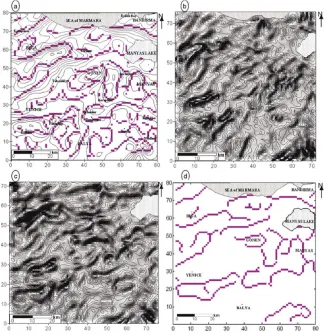
Here we choose CNN technique for determining the ge-ologic boundaries by virtual of the fact that it has various filtering characteristics owing to the cloning template. It is also widely used for residual-regional separation as well as border detection by choosing an appropriate cloning tem-plate. In this example, the Bouguer anomaly values of Biga and the surrounding areas are used in the CNN as input data, and the cloning template in Eq. (11) is used to detect geo-logic boundaries that are difficult to identify in the Bouguer anomaly map. CNN output is shown in Fig. 10(a). This map clearly shows that both major faults having large ver-tical displacements and minor faults that are not obvious in the Bouguer anomaly map are well defined using the CNN approach. The WNW-ESE trending strong gravity gradi-ent to the north of Manyas Lake (Fig. 9), extending also beneath the lake, shed light on a likely normal fault dip-ping SSW. Although the normal fault is not present on the active faults map of Turkey (S¸aro˘glu et al., 1992), there are several pieces of evidence supporting the existence of such a normal fault: (1) the regional stress tensor analysis based on focal mechanisms of earthquakes in the Marmara sea region indicate a NW-SE directed (1-axis and NE-SW trendingσ3-axis (Pinaret al., 2003) where one may expect a SSW-dipping normal fault; (2) the location and the pre-dominantly normal faulting mechanism with WNW-ESE-trending nodal planes of the 1964 Manyas-Karacabey earth-quake (Mw=6.6) suggest the existence of this normal fault (Eyido˘gan, 1991).
To compare the CNN method with classical derivative techniques, the CC method is also applied on the same
Bouguer anomaly map. The maxima or minima in the
Fig. 10. (a) Edge maps obtained by proposed approach, (b) gray-shaded relief of cross-correlation map in the E-W direction, (c) gray-shaded relief of cross-correlation map in the N-S direction, (d) edge map obtained by standard Canny algorithm. Cross-correlation maps are illuminated from the NW.
Figure 10(a)–(c) shows that the CNN and CC methods are similar in terms of their performance to detect major faults and minor faults. Thus, it can be concluded that the CNN is an effective method for detecting geologic boundaries, such as faults or the boundary of two geologic zones.
The CNN and the CC outputs shown in Fig. 10(a)– (c), which were obtained from the Bouguer anomaly map (Fig. 9), show that the position of faults generally correlate well with those of geological map of the region (Fig. 8). Many of the E-W- and NE-SW-trending faults in previously published geological maps (Elmas and Meric¸, 1998; Elmas, 2003; Smith et al., 1995; Okay et al., 1999; ˙Imrenet al., 2001; G¨ureret al., 2006; Figs. 7 and 8) are obvious in the CNN and CC outputs (Figs. 10(a)–(c)). On the other hand, the strike-slip fault that was ruptured by the 1953 Yenice-G¨onen earthquake (Figs. 7 and 8) was not detected in the CNN and CC outputs even though it is present in the geo-logical maps. We believe that this fault is not revealed in the processed data either because of insufficient and/or sparse data collection in the field or because the gravity data are not sensitive to lateral motions.
7.
Discussion and Conclusions
In this paper, an image processing technique called CNN approach is introduced as an approach for locating subsur-face geological features such as faults or the boundary of two geologic zones. CNN is a stochastic image processing
technique based on template optimization using the neigh-borhood relationships of cells. The network dynamic of a CNN is described by a set of differential equations. Each cell in a CNN has an input, an internal state and an output. The feedback control template represents the coupling coef-ficients of the cells, and this completely defines the behavior of the network with a given input and initial condition.
CNN is first applied on two synthetic data sets to detect the borders of vertical prismatic blocks, and the results are compared with those obtained with the CC technique. After satisfactory results had been verified, the proposed CNN algorithm is applied on the gravity anomaly map of Biga and surrounding area in Anotalia to evaluate the major and minor faults. The structural features in the area between Bandırma, Biga, Yenice and Gonen in the southwestern Marmara region are investigated by applying the CNN and CC algorithms to the Bouguer anomaly map. As shown in Fig. 10(a), the CNN output provides a better visualization of the outlines of the geologic features. The results of the proposed approach (Fig. 10(a)) are in good agreement with previously observed faults in the field (Elmas and Meric¸, 1998; Elmas, 2003; Smithet al., 1995; Okayet al., 1999; ˙Imrenet al., 2001; G¨ureret al., 2006; Figs. 7 and 8). It is shown that the CNN and CC methods are similar in terms of their performance in detecting geologic boundaries.
south-It would seem that the structural results and the tectonic map of the region, the latter of which was prepared by ap-plying the CNN method to the gravity anomaly map, are predominantly in accordance with the results of previous field studies. Moreover, the use of this method provides a more detailed general view of structural features. For ex-ample, the strongly gravity anomaly to the north of Manyas Lake (Fig. 9) indicates the existence of a fault which dis-plays a progressive change in trend from NW in the east to E-W in the west. The fault has not been identified by previous field studies.
Consequently, by applying the proposed approach to the Bouguer anomaly map, a detailed general view of surface and subsurface structural boundaries can be obtained suc-cessfully. The CNN method, as applied to the location of edges of causative sources, is simple and easy to use and is a good approach for determining vertical or near vertical faults. Thus, this method can be a useful geophysics tool for investigating structural boundaries over wide areas.
Acknowledgments. I would like to express my thanks to Dr. Takeshi Sagiya (Editor and reviewer) and Dr. Masao Komazawa (reviewer) for their very careful reading, valuable comments, mod-ifications and suggestions. I thank Dr. Ali Elmas, Dr. Ali Pınar and Dr. Aysan G¨urer for their very careful reading and suggestions on the text.
References
Altınlı, ˙I. E., The geology of middle Sakarya, Congress Proceeding of Earth Sciences 50th Anniversary of Turkish Republic. Min. Res. and Exp. Inst. (M.T.A), Ankara, 159–191, 1973 (in Turkish).
Aydogan, D., A. Elmas, A. M. Albora, and O. N. Ucan, A new approach to the structural features of the Aegean Sea: Cellular neural network,Mar. Geophys. Res.,26, 1–15, 2005.
Barka, A. A., The North Anatolian fault zone,Annales Tectonicae,6, 164– 195, 1992.
Barka, A. A. and K. Kadinsky-Cade, Strike-slip fault geometry in Turkey and its influence on earthquake activity,Tectonics,7, 663–684, 1988. Bing¨ol, E., B. Aky¨urek, and B. Korkmazer, The geology of Biga Peninsula
and the features of Karakaya Formation, Congress Proc of Earth Sci 50th Anniversary of Turkish Republic: Min. Res. and Explor. Inst., Ankara, 70–77, 1973 (in Turkish).
Blakely, R. J. and R. W. Simpson, Approximating edges of source bodies from magnetic or gravity anomalies,Geophysics,51(7), 1494–1498, 1986.
Boschetti, F., Improved edge detection and noise removal in gravity maps via the use of gravity gradients,J. Appl. Geophys.,57, 213–225, 2005. Canny, J., A computational approach to edge detection,IEEE Transaction
on Pattern Analysis and Machine Intelligence PAMI,8(6), 679–698, 1986.
Chua, L. O. and L. Yang, Cellular neural networks: Theory,IEEE Trans-action on Circuits and Systems,35(10), 1257–1272, 1988a.
Chua, L. O. and L. Yang, Cellular neural networks: Applications,IEEE Transaction on Circuits and Systems,35(10), 1273–1290, 1988b. Dewey, J. F., M. Hempton, W. Kidd, F. S¸aro˘glu, and A. M. C. S¸eng¨or,
Shortening of continental lithosphere: the neotectonics of eastern Ana-tolia: a young collision zone, inCollision tectonics, edited by M. P. Coward and A. C. Ries,Geol. Soc. Lond. Spec. Publ.,19, 3–36, 1986. Dewey, J. F. and A. M. C. S¸eng¨or, Aegean and surrounding regions:
com-plexmultiplate and continuum tectonics inaconvergent zone,Geol. Soc. Am. Bull.,90, 84–92, 1979.
G¨or¨ur, N. (ed.), Kuzey Ege, Marmara Denizi ve dolayının jeolojisi deniz yapılas¸malarındaki ¨onemi Kolokyumu. ˙IT ¨U Extended abstracts 7–17, 1997.
Eyido˘gan, H., Z. Utku, U. G¨uc¸l¨u, and E. De˘girmenci, The macroseismic guidance of the large Turkish earthquakes (1900–1988), ITU, Istanbul, 1991.
Fedi, M. and G. Florio, Detection of potential fields source boundaries by enhanced horizontal derivative method,Geophys. Prospect.,49, 40–58, 2001.
G¨urer, ¨O. F., N. Kaymakc¸ı, S¸. C¸ akır, and M. ¨Ozburan, Neotectonics of the southeast Marmara region, NW Anatolia, Turkey,J. Asian Earth Sci., 21, 1041–1051, 2003.
G¨urer, ¨O. F., E. Sangu, and M. ¨Ozburan, Neotectonics of the SW Marmara region, NW Anatolia, Turkey,Geol. Mag.,143(2), 1–13, 2006. ˙Imren, C., X. Le Pichon, C. Rangin, E. Demirba˘g, B. Ecevito˘glu, and N.
G¨or¨ur, The North Anatolian Fault within the Sea of Marmara, A new in-terpretation based on multi-channel seismic and multi-beam bathymetry data,Earth Planet. Sci. Lett.,186, 143–158, 2001.
Jackson, J. and D. P. McKenzie, The relationship between plate motions and seismic moment tensors and the rates of active deformation in the Mediterranean and Middle East,Geophys. J.,93, 45–73, 1988. Ketin, ˙I., About of the North Anatolian Fault,Bull. Min. Res. Expl. Inst.,
Turkey,72, 1–25, 1969.
Letouzey, J., B. Bıju-Duval, A. Dorkel, R. Gonnard, K. Kristchev, L. Mon-tadert, and O. Sungurlu, The Black Sea: a marginal basin, Geophysi-cal and geologiGeophysi-cal data, inInternational Symposium on the Structural History of the Mediterranean Basins, edited by B. Bıju-Duval and L. Montadert, 363–376, 1977, Editions Technip (Paris).
McKenzie, D. P., Active tectonics of the Mediterranean region,Geophys. JR. Astron. Soc.,30, 109–185, 1972.
Okay, A. I., E. Demirba˘g, H. Kurt, N. Okay, and ˙I. Kus¸c¸u, An active, deep marine strike-slip basin along the North Anatolian Fault in Turkey,
Tectonics,18, 129–147, 1999.
Pınar, A., Y. Honkura, and K. Kuge, Moment tensor inversion of recent small to moderate sized earthquakes: Implication for seismic hazard and active tectonics beneath the Sea of Marmara,Geophys. J. Int.,152, 133– 145, 2003.
Reid, A. B., J. M. Allsop, H. Granser, A. J. Millett, and I. W. Somerton, Magnetic interpretation in three dimensions using Euler deconvolution,
Geophysics,55, 80–91, 1990.
Sahbaz, A., M. ¨Ozdo˘gan, S. G¨orm¨us¸, and E. Bayhan, Sedimentology of Mudanya formation: depositional processes controlling the develop-ment of Gilbert type fan delta (Middle-Late Miocene, South of Marmara Sea),Yerbilimleri,20, 111–122, 1998.
Smith, A. D., T. Taymaz, F. Oktay, H. Y¨uce, B. Alpar, H. Bas¸aran, A. J. Jackson, S. Kara, and M. S¸ims¸ek, High-resolution seismic profiling in the Sea of Marmara: Late Quaternary sedimentation and sea-level changes,Geol. Soc. Am. Bull.,107, 923–936, 1995.
Sykes, M. P. and U. C. Das, Directional filtering for linear feature enhance-ment in geophysical maps,Geophysics,65, 1758–1768, 2000. S¸aro˘glu, F., ¨O. Emre, and ˙I. Kus¸u, Active fault map of Turkey, MTA, 1992. S¸eng¨or, A. M. C., The North Anatolian transform fault: its age, offset and
tectonic significance,J. Geol. Soc. Lond.,136, 269–282, 1979. S¸eng¨or, A. M. C., N. G¨or¨ur, and F. S¸aro˘glu, Strike-slip faulting and related
basin formation in zones of tectonic escape: Turkey as a case study, in
Strike-slip Basin Formation and Sedimentation, edited by K. T. Biddle and N. Christie-Blick,Soc. Econ. Paleon. Min. Spec. Publ.,37, 227– 264, 1985.
Thompson, D. T., EULDPH: A new technique for making computer-assisted depth estimates from magnetic data,Geophysics,47, 31–37, 1982.
Zeng, H., Q. Zhang, and J. Liu, Location of secondary faults from cross-correlation of the second vertical derivative of gravity anomalies, Geo-phys. Prospect.,42, 841–854, 1994.