R E S E A R C H
Open Access
Adaptive dynamic surface control of
parametric uncertain and disturbed
strict-feedback nonlinear systems
Chenhui Wang
1**Correspondence: [email protected] 1College of Applied Mathematics,
Xiamen University of Technology, Xiamen, China
Abstract
The construction of backstepping control input needs the derivative of the virtual controller to be available. However, this requirement usually makes the
implementation of the controller very difficult and complicated. To overcome this problem, in this paper, an adaptive dynamic surface control (ADSC) is proposed for a class of strict-feedback nonlinear systems with parametric uncertainty and external disturbance. In each step of the backstepping control design, the virtual control input is estimated by an auxiliary signal which is generated by a proposed dynamic surface. This signal’s derivative is easy to obtain, so it is not necessary to achieve the derivative of the virtual control input. By using the Lyapunov stability theorem, an ADSC has been established to guarantee the boundedness of all signals and the convergence of the tracking errors. Finally, a simulation example is given to indicate the
effectiveness of our control approach.
Keywords: Strict-feedback nonlinear system; Adaptive backstepping control; Adaptive dynamic surface control; Mismatched uncertainty
1 Introduction
It is well known that tremendous success has been obtained in controlling nonlinear sys-tems based on the development of adaptive backstepping control (ABC) and feedback linearization (FBL) methods [1,2]. The main idea of FBL consists in transforming a strict-feedback nonlinear system (SFNS) that satisfies some matching conditions into a linear one. That is to say, this method cannot deal with the nonlinear term directly. To overcome this limitation, the ABC method establishes a systematic framework for controlling SFNSs, whose main idea is using some intermediate variables recursively as pseudo-control sig-nals. If the SFNSs have minimum phase and have known relative degrees, the stability of the closed-loop system can be guaranteed by using the backstepping design method. For ABC of an SFNS without parametric uncertainty or external disturbance, some control methods have been presented, for example, in [2–5]. Based on the main idea of the ABC approach, more complicated conditions are considered in designing ABC for SFNS in [2,
6–8]. However, the above literature did not consider parametric uncertainties and distur-bance in the ABC design. Thus, the ABC design needs to be studied further to achieve better robust performance.
As is well known, most physical systems usually suffer from system uncertainty, for ex-ample, parametric uncertainty, modeling error, or external disturbance, which will de-crease the control performance or even leads to instability of the controlled system [9–
21]. Thus, the ABC method usually requires cancelation of the nonlinearities. Sometimes exact knowledge of the system nonlinearities is not available, or these terms change along with time. Therefore, we need to model the nonlinear uncertainties with parametric un-certainties. Some robust control methods have been given to handle these kinds of system uncertainties [19,22–39]. ABC methods have been studied recently in [40–42]. In [2], an ABC method combined with adaptive fuzzy control was investigated. A fuzzy ABC for SFNSs in the presence of both sampled and delayed measurements was studied in [40]. A command filtered ABC method for unknown SFNSs was proposed in [41], where a first-order filter was introduced to handle the virtual control input. However, in the above literature, external disturbance and/or parametric uncertainty was not considered.
The ABC method suffers from the “explosion of complexity” which is produced by re-peatedly differentiating the virtual control input. Then, many control methods have been given to solve this problem. Among these, the adaptive dynamic surface control (ADSC) aims to enhance the drawback of ABC by driving the control input passing through a first-order filter [23,43–46]. This method not only solve the problem of “explosion of complex-ity”, but also reduce the requirement of the system model as well as the referenced signal. In [23], by using the ADSC method, an ABC method was proposed for SFNSs with para-metric uncertainties. Reference [47] provides a command filtered backstepping control for SFNSs, where the adaptive control method was not considered. Then, based on the work of [47], Ref. [22] provided an adaptive command filtered backstepping control method, and a compensated tracking error was also considered. The above method is based on pro-cedures like nonlinear damping and variable structure as well as their variations, which commonly need prior knowledge of the system uncertainty, for example, utilizing some constant or nonlinear function known in advance as the bounds of the estimated nonlin-earity. Consequently, the applications of these kinds of methods may be limited if there is no such prior knowledge.
2 Problem formulation
Consider the followingnth parametric uncertain SFNSs:
⎧ ⎨ ⎩ ˙
xi(t) =xi+1(t) +fi(xxx¯i(t)) +ϕϕϕTi(xxx¯i(t))ϑϑϑ, i= 1, 2, . . . ,n– 1,
˙
xn(t) =fn(xxx(t)) +d(t) +u(t) +ϕϕϕTn(xxx¯(t))ϑϑϑ, (1)
where x1(t)∈Ris the output variable, u(t)∈Ris the control input,xxx¯i(t) = [x1(t), . . . ,
xi(t)]T ∈Ri (note that xxx(t) =xxx¯n(t)∈Rn) represents the system state vector, fi(xxx¯i(t)): Ri→Ris a nonlinear function,d(t)∈Rdenotes the bounded unknown external distur-bance,ϕϕϕi(xxx¯i(t)):Ri→Rmis a known basis function, andϑϑϑ= [ϑ
1, . . . ,ϑm]∈Rmrepresents
an unknown constant vector.
Define xd(t)∈Ras a desired signal. The main objective of this paper is to design an ADSC such that the output variablex1(t) follows the desired signalxd(t). Let the tracking
error be
e1(t) =x1(t) –xd(t). (2)
Throughout this paper,R,Rirepresent the spaces of real numbers and reali-vectors, respectively.x(t)is the standard 2-norm ofx(t),sgn(·) denotes the signum function,L∞
represents the space of the bounded variable,Ωcis the ball of radiusc, andCiis the space of functions for which allith-order derivatives exist and are continuous.
To facilitate the controller design, we need the following assumptions.
Assumption 1 The nonlinear functionsfi(xxx¯(t)),ϕϕϕn(xxx¯(t)) are ofC1.
Assumption 2 The desired signalxd(t) and its derivative are continuous functions ofL∞.
Assumption 3 The external disturbanced(t) is bounded, i.e., there exists a positive con-stantd∗such that|d(t)| ≤d∗.
Assumption 4 Assume thatΩcis an open set which includes the referenced signal, the origin and the initial conditions of the system 1. Suppose that, for i= 1, . . . ,n, ∂jfi(xxx¯i(t))
∂tj ,
∂jx d(t)
∂tj , wherej= 1, . . . ,n, are all bounded onΩ¯c.
Remark1 It is worth mentioning that above four assumptions are in line with the practical situation. Firstly, the Assumption1is satisfied in most real-world systems. Secondly, in most literature, the referenced signal is a smooth function, that is to say, Assumption2
is reasonable. Thirdly, in this paper, it is assumed that the unknown external disturbance
d(t) is bounded. In fact, lots of common disturbance functions are bounded. In addition, the upper boundd∗is assumed to be unknown. Finally, Assumption4is needed in the stability analysis, and this assumption is common in much related literature, for example, [22,23,47].
3 Controller design and stability analysis
3.1 The ADSC design
Step 1.
whereν1(t) represents the virtual control input that will be defined later,
e2(t) =x2(t) –ν1c(t) (4)
is the filtered tracking error ofx2(t), andν˜1(t) =ν1c(t) –ν1(t) denotes the virtual control
input estimation error. Thus, the virtual control inputν1(t) can be given as
ν1(t) = –k1e1(t) –f1
whereσ1> 1 is a design parameter.
and the virtual control inputν2(t) can be constructed as
These steps are very similar to Step 2. It is easy to see that
˙
and the virtual control inputνi(t) can be constructed as
νi(t) = –kiei(t) –ei–1(t) –fi
¯
xxxi(t)–ϕϕϕTi xxx¯i(t)ϑϑϑ(ˆ t) +ν˙ic–1(t), (14)
whereki> 0 andσi> 1 are two design parameters. Substituting (14) into (12) yields
In the final step, the control inputu(t) will be constructed. Based on the discussion in Stepn– 1, we have
Then the control input can be given as
u(t) = –knen(t) –fn
xxx(t)–ϕϕϕTnxxx¯(t)ϑϑϑ(ˆ t) +ν˙nc–1(t) –dˆ∗(t)signen(t)–en–1, (17)
wherekn> 0 is a design parameter,dˆ∗(t) is the estimation of the unknown positive constant
d∗. Then, (16) and (17) implies
˙
en(t) = –knen(t) +d(t) –dˆ∗(t)sign
3.2 Stability analysis
The proposed filters, i.e., (6), (9), (13) can guarantee thatν˜i(t) is sufficiently small eventu-ally. To prove this result, we give the following lemma first.
Lemma 1 Suppose that z(t)satisfies|z(t)| ≤β,|˙z(t)| ≤γ and
˙
y(t) = –wy(t) –z(t), y(0) =z(0), (19)
where w> 0.Then we have|y(t) –z(t)| ≤ γw.
Proof Denotey˜(t) =y(t) –z(t). It is easy to see that(0) = 0. Then we have
˙˜
y(t) = –wy˜(t) –z˙(t). (20)
The solution of (20) can be given as
˜ y(t) = –
t
0
˙
z(t)e–w(τ–t)dτ. (21)
Thus, we have
y˜(t)=
t
0
˙
z(t)e–w(τ–t)dτ
≤ t
0
z˙(t)e–w(τ–t)dτ
≤γ
t
0
e–w(τ–t)dτ
=γ
w
1 –e–wt. (22)
Thus,|y(t) –z(t)| ≤γw, and this ends the proof of Lemma1. Based on above result, we can easily obtain the following theorem.
Theorem 1 Under Assumptions3and4,we see that,for anyμi> 0,there exists a constant
T> 0,for all t>T,|˜νi(t)| ≤μiif sufficiently large parametersσiare chosen.
Proof Based on (6), (9), (13), Assumptions3and4, and Lemma1, we know that fori= 1, . . . ,nand anyμi> 0
ν˜i(t)=νic(t) –νi(t)≤μi (23)
if sufficiently largeσiis chosen.
Now, let us give the following main results.
designed as
= – The Lyapunov function is defined as
V(t) =1
2is a positive constant.
Ac-cording to the Lyapunov stability criterion, we know that (31) implied thateee(t) ≤
enough, too. Thus, the tracking errorsei(t) will eventually converge to a small region at
zero ifαis small enough.
Remark2 From the results of Theorem2we know that to drive the tracking errorsei(t) small enough, we should choose small enoughμi,λ12andλ22. We know thatμiwill be
arbitrarily small ifσiare chosen large enough. With respect toλ12andλ22, in some
this case that the boundedness of the updated parameters cannot be guaranteed. Thus, in our method, these parameters are introduced for the purpose to guarantee the bound-edness of all signals in the closed-loop system. In the simulation, to achieve good control performance, we can set these parameters sufficiently small.
Remark3 In this paper, the dynamic surfaces (6), (10) and (14) are used to get the esti-mation of the virtual control inputs and their derivatives. It should be mentioned that the proposed Lemma1plays an important role in the stability analysis, which can guarantee the estimation error to be as small as possible. The estimation error can be adjusted by the design parameterσi. In fact, in practical applications, one does not to select too large σi, which is indicated by the following simulation results.
Remark4 In the conventional ABC method, every middle variable is treated as an input, and by using Lyapunov stability theorems, a virtual control input is designed. In the next step, the derivative of the virtual input is needed. However, as the order increases, it is more and more difficult to get the exact value of the derivative of the virtual input. Thus, the “explosion of complexity” occurs. To overcome this problem, in [2,40–42], the deriva-tive of the virtual input was estimated by using a fuzzy logic system, however, more control energy is needed and more computational burden will be added to the control system. In this paper, the ADSC method was proposed for SFNS with parametric uncertainty. The ADSC is an extension of the ABC, which is effective for handling SFNS. By using the pro-posed dynamical surface, i.e. (6), (10) and (14), the estimation of the derivatives of the virtual inputs is easy to obtain. As a result, the “explosion of complexity” problem can be solved effectively.
4 Simulation example
To indicate the effectiveness of the proposed control method, the well-known Chua chaotic system will be used in the simulation, which can be described as [20]
⎧ ⎪ ⎪ ⎨ ⎪ ⎪ ⎩ ˙
x1(t) = 11.25x2(t) – 11.25x1(t) –f(x1(t)),
˙
x2(t) =x3(t) +x1(t) –x2(t) +ϕϕϕT2(xxx¯2(t))ϑϑϑ,
˙
x3(t) = 18.6x2(t) +d(t) +u(t),
(32)
with
fx1(t)
= –0.68x1(t) – 0.545x1(t) + 1–x1(t) – 1.
In system (32),ϕϕϕ1(x1(t)) =ϕϕϕ3(xxx(t))≡0. The uncontrolled and undisturbed system (32)
(i.e.,u(t) =d(t) = 0,ϕϕϕ2(xxx¯2(t)) = 000) shows chaotic behavior, which is depicted in Fig.1.
In the simulation, letϑϑϑ= [1.5, 2.1, –1.5]T,ϕϕϕ
2(xxx¯2(t)) = [x1(t),x2(t),x1(t)sinx2(t)]T, and the
disturbance is set asd(t) = 0.5sint. The referenced signalxd(t) and its first-order derivative is produced by the following differential equation:
˙
ζζζ(t) =
0 1
–25 –10
ζζζ(t) +
0 25
ζc(t), (33)
whereζζζ(0) = [0, 0]T,ζc(t) =π/6 fort∈[0, 5] andζc(t) = 0 fort> 5 withxd(t) =ζ
1(t) and
˙
Figure 1Chaotic behavior of system (32) under initial conditionxxx(0) = [1.6, –1.1, 0.7]
Figure 2 x1(t) andxd(t)
The controller design parameters are chosen ask1=k2=k3= 1.5, σ1=σ2=σ3= 20,
λ11 =λ21= 10,λ21 =λ22= 0.05. The true value ofϑϑϑ isϑϑϑ= [–0.5, 0.1, 0.5]T. The initial
conditions forϑϑϑ(ˆ t) anddˆ∗(t) areϑϑϑ(0) = 0ˆ 00 anddˆ∗(0) = 0, respectively.
Figures2–6 depict the simulation results. The tracking performance is indicated in Fig.2, from which we can see that the output variablex1(t) of system (32) follows the
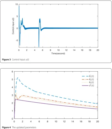
Figure 3Control inputu(t)
Figure 4The updated parameters
method guarantee a fast convergence of the tracking error. The time response of the con-trol inputu(t) is shown in Fig.3. It should be pointed out that the chattering phenomenon can be seen in Fig.3because the sign function is included in the proposed controller (17). In fact, to cancel the chattering, we can replace the sign function with some continuous function, such as thearctanfunction. The updated parametersϑˆ1(t),ϑˆ2(t),ϑˆ3(t) anddˆ∗(t)
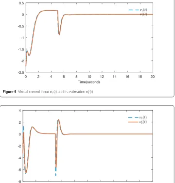
are presented in Fig.4, from which we can see that the boundedness of these parame-ters can be guaranteed. Finally, the tracking performance betweenν1(t)(t) andν1c(t), and
ν2(t)(t) andν2c(t) is given in Fig.5and Fig.6, respectively. It is indicated that the proposed
dynamic surfaces have very good estimation ability.
5 Conclusions
Figure 5Virtual control inputν1(t) and its estimationν1c(t)
Figure 6Virtual control inputν2(t) and its estimationν2c(t)
the controlled system suffers from parametric uncertainty and external disturbances. It has been proven that our method is feasible for a wider range of SFNSs than conventional ABC and the dynamic surface can also be utilized to enhance constraints on the state tra-jectories. The proposed ADSC guarantees that all signals in the closed-loop system keep bounded and tracking errors converge to a sufficiently small region. The effectiveness of our method has been verified by a simulation results. Our future research direction in-clude: (1) Design an extended controller consider how to deduce the requirement of the system model; (2) Combined our method with some robust control approach, for example, adaptive fuzzy control, adaptive neural network control, sliding mode control.
Acknowledgements
Not applicable.
Funding
Competing interests
The authors declare that they have no competing interests.
Authors’ contributions
All authors contributed equally to the writing of this paper. All authors conceived of the study, participated in its design and coordination, read and approved the final manuscript.
Publisher’s Note
Springer Nature remains neutral with regard to jurisdictional claims in published maps and institutional affiliations.
Received: 31 August 2018 Accepted: 15 January 2019
References
1. Krstic, M., Kanellakopoulos, I., Kokotovic, P.V., et al.: Nonlinear and Adaptive Control Design, vol. 222. Wiley, New York (1995)
2. Liu, H., Pan, Y., Li, S., Chen, Y.: Adaptive fuzzy backstepping control of fractional-order nonlinear systems. IEEE Trans. Syst. Man Cybern. Syst.47(8), 2209–2217 (2017)
3. Li, H., Wang, L., Du, H., Boulkroune, A.: Adaptive fuzzy backstepping tracking control for strict-feedback systems with input delay. IEEE Trans. Fuzzy Syst.25(3), 642–652 (2017)
4. Coron, J.-M., Hu, L., Olive, G.: Finite-time boundary stabilization of general linear hyperbolic balance laws via Fredholm backstepping transformation. Automatica84, 95–100 (2017)
5. Chen, C.P., Wen, G.-X., Liu, Y.-J., Liu, Z.: Observer-based adaptive backstepping consensus tracking control for high-order nonlinear semi-strict-feedback multiagent systems. IEEE Trans. Cybern.46(7), 1591–1601 (2016) 6. Kwan, C., Lewis, F.L.: Robust backstepping control of nonlinear systems using neural networks. IEEE Trans. Syst. Man
Cybern., Part A, Syst. Hum.30(6), 753–766 (2000)
7. Vaidyanathan, S., Volos, C., Pham, V.-T., Madhavan, K., Idowu, B.A.: Adaptive backstepping control, synchronization and circuit simulation of a 3-d novel jerk chaotic system with two hyperbolic sinusoidal nonlinearities. Arch. Control Sci.
24(3), 375–403 (2014)
8. Li, Y., Sui, S., Tong, S.: Adaptive fuzzy control design for stochastic nonlinear switched systems with arbitrary switchings and unmodeled dynamics. IEEE Trans. Cybern.47(2), 403–414 (2017)
9. Wu, H.: Liouville-type theorem for a nonlinear degenerate parabolic system of inequalities. Math. Notes Acad. Sci. USSR103(1–2), 155–163 (2018)
10. Hao, X., Zuo, M., Liu, L.: Multiple positive solutions for a system of impulsive integral boundary value problems with sign-changing nonlinearities. Appl. Math. Lett.82, 24–31 (2018)
11. Wang, P., Liu, X., Liu, Z.: The convexity of the level sets of maximal strictly space-like hypersurfaces defined on 2-dimensional space forms. Nonlinear Anal.174, 79–103 (2018)
12. Peng, X., Shang, Y., Zheng, X.: Lower bounds for the blow-up time to a nonlinear viscoelastic wave equation with strong damping. Appl. Math. Lett.76, 66–73 (2018)
13. Sun, W.W.: Stabilization analysis of time-delay Hamiltonian systems in the presence of saturation. Appl. Math. Comput.217(23), 9625–9634 (2011)
14. Sun, W., Peng, L.: Observer-based robust adaptive control for uncertain stochastic Hamiltonian systems with state and input delays. Nonlinear Anal., Model. Control19(4), 626–645 (2014)
15. Guo, Y.: Exponential stability analysis of travelling waves solutions for nonlinear delayed cellular neural networks. Dyn. Syst.32(4), 490–503 (2017)
16. Xu, Y., Zhang, H.: Positive solutions of an infinite boundary value problem for nth-order nonlinear impulsive singular integro-differential equations in Banach spaces. Appl. Math. Comput.218(9), 5806–5818 (2012)
17. Liu, C., Wu, X.: The boundness of the operator-valued functions for multidimensional nonlinear wave equations with applications. Appl. Math. Lett.74, 60–67 (2017)
18. Lin, X., Zhao, Z.: Iterative technique for third-order differential equation with three-point nonlinear boundary value conditions. Electron. J. Qual. Theory Differ. Equ.2016, 12 (2016)
19. Pan, Y., Yu, H.: Biomimetic hybrid feedback feedforward neural-network learning control. IEEE Trans. Neural Netw. Learn. Syst.28(6), 1481–1487 (2017)
20. Liu, H., Li, S., Wang, H., Huo, Y., Luo, J.: Adaptive synchronization for a class of uncertain fractional-order neural networks. Entropy17(10), 7185–7200 (2015)
21. Liu, H., Li, S., Wang, H., Sun, Y.: Adaptive fuzzy control for a class of unknown fractional-order neural networks subject to input nonlinearities and dead-zones. Inf. Sci.454–455, 30–45 (2018)
22. Dong, W., Farrell, J.A., Polycarpou, M.M., Djapic, V., Sharma, M.: Command filtered adaptive backstepping. IEEE Trans. Control Syst. Technol.20(3), 566–580 (2012)
23. Pan, Y., Yu, H.: Composite learning from adaptive dynamic surface control. IEEE Trans. Autom. Control61(9), 2603–2609 (2016)
24. Li, F., Gao, Q.: Blow-up of solution for a nonlinear Petrovsky type equation with memory. Appl. Math. Comput.274, 383–392 (2016)
25. Gao, L., Wang, D., Wang, G.: Further results on exponential stability for impulsive switched nonlinear time-delay systems with delayed impulse effects. Appl. Math. Comput.268, 186–200 (2015)
26. He, X., Qian, A., Zou, W.: Existence and concentration of positive solutions for quasilinear Schrödinger equations with critical growth. Nonlinearity26(12), 3137 (2013)
27. Feng, Y.-H., Liu, C.-M.: Stability of steady-state solutions to Navier–Stokes–Poisson systems. J. Math. Anal. Appl.462(2), 1679–1694 (2018)
29. Cao, X., Wang, J.: Finite-time stability of a class of oscillating systems with two delays. Math. Methods Appl. Sci.41(13), 4943–4954 (2018)
30. Shen, T., Xin, J., Huang, J.: Time–space fractional stochastic Ginzburg–Landau equation driven by Gaussian white noise. Stoch. Anal. Appl.36(1), 103–113 (2018)
31. Li, M., Wang, J.: Exploring delayed Mittag-Leffler type matrix functions to study finite time stability of fractional delay differential equations. Appl. Math. Comput.324, 254–265 (2018)
32. Liu, S., Wang, J., Zhou, Y., Feˇckan, M.: Iterative learning control with pulse compensation for fractional differential systems. Math. Slovaca68(3), 563–574 (2018)
33. Zhang, J., Wang, J.: Numerical analysis for Navier–Stokes equations with time fractional derivatives. Appl. Math. Comput.336, 481–489 (2018)
34. Zhang, J., Lou, Z., Ji, Y., Shao, W.: Ground state of Kirchhoff type fractional Schrödinger equations with critical growth. J. Math. Anal. Appl.462(1), 57–83 (2018)
35. Wang, Y., Jiang, J.: Existence and nonexistence of positive solutions for the fractional coupled system involving generalized p-Laplacian. Adv. Differ. Equ.2017(1), 337 (2017)
36. Feng, Q., Meng, F.: Traveling wave solutions for fractional partial differential equations arising in mathematical physics by an improved fractional Jacobi elliptic equation method. Math. Methods Appl. Sci.40(10), 3676–3686 (2017) 37. Hao, X.: Positive solution for singular fractional differential equations involving derivatives. Adv. Differ. Equ.2016(1),
139 (2016)
38. Diblík, J., Feckan, M., Pospíšil, M.: On the new control functions for linear discrete delay systems. SIAM J. Control Optim.52(3), 1745–1760 (2014)
39. Diblík, J., Khusainov, D.Y., Baštinec, J., Sirenko, A.: Exponential stability of linear discrete systems with constant coefficients and single delay. Appl. Math. Lett.51, 68–73 (2016)
40. Wang, T., Zhang, Y., Qiu, J., Gao, H.: Adaptive fuzzy backstepping control for a class of nonlinear systems with sampled and delayed measurements. IEEE Trans. Fuzzy Syst.23(2), 302–312 (2015)
41. Wang, Y., Cao, L., Zhang, S., Hu, X., Yu, F.: Command filtered adaptive fuzzy backstepping control method of uncertain non-linear systems. IET Control Theory Appl.10(10), 1134–1141 (2016)
42. Sadek, U., Sarjaš, A., Chowdhury, A., Sveˇcko, R.: Improved adaptive fuzzy backstepping control of a magnetic levitation system based on symbiotic organism search. Appl. Soft Comput.56, 19–33 (2017)
43. Zhai, D., Xi, C., An, L., Dong, J., Zhang, Q.: Prescribed performance switched adaptive dynamic surface control of switched nonlinear systems with average dwell time. IEEE Trans. Syst. Man Cybern. Syst.47(7), 1257–1269 (2017) 44. Singh, U.P., Jain, S., Singh, R., Parmar, M., Makwana, R., Kumare, J.: Dynamic surface control based ts-fuzzy model for a
class of uncertain nonlinear systems. Int. J. Control Theory Appl.9(2), 1333–1345 (2016)
45. Uyen, H.T.T., Tuan, P.D., Van Tu, V., Quang, L., Minh, P.X.: Adaptive neural networks dynamic surface control algorithm for 3 dof surface ship. In: System Science and Engineering (ICSSE), 2017 International Conference on, pp. 71–76. IEEE (2017)
46. Semprun, K.A., Yan, L., Butt, W.A., Chen, P.C.: Dynamic surface control for a class of nonlinear feedback linearizable systems with actuator failures. IEEE Trans. Neural Netw. Learn. Syst.28(9), 2209–2214 (2017)
47. Farrell, J., Sharma, M., Polycarpou, M.: Backstepping-based flight control with adaptive function approximation. J. Guid. Control Dyn.28(6), 1089–1102 (2005)
48. Pan, Y., Yu, H.: Dynamic surface control via singular perturbation analysis. Automatica57, 29–33 (2015) 49. Ma, J., Zheng, Z., Li, P.: Adaptive dynamic surface control of a class of nonlinear systems with unknown direction
control gains and input saturation. IEEE Trans. Cybern.45(4), 728–741 (2015)
50. Zhang, X., Liu, L., Wu, Y.: The uniqueness of positive solution for a fractional order model of turbulent flow in a porous medium. Appl. Math. Lett.37, 26–33 (2014)
51. Wang, J., Yuan, Y., Zhao, S.: Fractional factorial split-plot designs with two-and four-level factors containing clear effects. Commun. Stat., Theory Methods44(4), 671–682 (2015)
52. Zhang, L., Zheng, Z.: Lyapunov type inequalities for the Riemann–Liouville fractional differential equations of higher order. Adv. Differ. Equ.2017(1), 270 (2017)
53. Liu, H., Pan, Y., Li, S., Chen, Y.: Synchronization for fractional-order neural networks with full/under-actuation using fractional-order sliding mode control. Int. J. Mach. Learn. Cybern.9(7), 1219–1232 (2018)
![Figure 1 Chaotic behavior of system (32) under initial condition xxx(0) = [1.6,–1.1,0.7]](https://thumb-us.123doks.com/thumbv2/123dok_us/937643.1114084/10.595.119.479.79.384/figure-chaotic-behavior-initial-condition-xxx.webp)