Operator compact exponential approximation for the solution of the system of 2D second order quasilinear elliptic partial differential equations

(1)

R E S E A R C H

Open Access

Operator compact exponential

approximation for the solution of the system

of 2D second order quasilinear elliptic partial

differential equations

R.K. Mohanty

1*

_{, Geetan Manchanda}

2,3

_{and Arshad Khan}

2

*_{Correspondence:} [email protected] 1_{Department of Applied}

Mathematics, South Asian University, New Delhi, India Full list of author information is available at the end of the article

Abstract

In this paper, we suggest a new exponential implicit method based on full step discretization of order four for the solution of quasilinear elliptic partial diﬀerential equation of the formA(x,y,z)zxx+C(x,y,z)zyy=k(x,y,z,zx,zy), 0 <x,y< 1. In this method a single compact cell consisting of nine nodal points is used. Convergence analysis of the said method is discussed in detail. The developed method is

successfully applied to solving problems in polar coordinates. The method for scalar equation is eventually applied to solving the system of quasilinear elliptic equations. To measure the rationality and precision, the method is applied to solving several noteworthy problems and numerical results are provided to exhibit the eﬀectiveness of the method.

MSC: 65N06; 65N12

Keywords: Quasilinear elliptic equations; Compact exponential approximation; Fourth order diﬀerence methods; Convergence analysis; Burger’s equation; Convection-diﬀusion equation; Navier–Stokes equations of motion

1 Introduction

We examine a quasilinear elliptic equation in two space dimensions of the form

A(x,y,z)zxx+C(x,y,z)zyy=k(x,y,z,zx,zy), (1.1)

where (x,y)∈Γ = (0, 1)×(0, 1).

z(x,y) =z0(x,y), (x,y)∈∂Γ. (1.2)

The partial differential equations (PDEs) of the type (1.1) with non-constant coefficients illustrate several real world problems of phenomenological importance like Poisson’s equation, convection–diffusion equation, Burgers’ equation and the nonlinear steady-state Navier–Stokes (NS) equations of motion.

We presuppose the following about the boundary value problem (1.1)–(1.2):

(2)

1. A.C> 0inΓ, 2. z(x,y)∈C6, 3. A,C∈C4_, 4. kis continuous, 5. ∂_∂k_z ≥0,

6. |∂k ∂zx| ≤H,|

∂k ∂zy| ≤I,

whereHandIare ﬁnite positive real bounds andCp_{is the class of functions with smooth} partial derivatives up to orderp(Jainet al. [1]).

The ellipticity condition of Eq. (1.1) is ensured by (1). Assumptions (2)–(4) are required to enable the Taylor series expansions, and (5)–(6) are the adequate conditions for the existence and uniqueness of the solution of the boundary value problem (1.1)–(1.2) (Jain

et al. [2]).

Elliptic equations, a type of partial differential equations illustrate behavior that remains static with time. In other words processes which are in equilibrium, like heat flow or fluid flow through a medium without any accumulations. The elliptic equation satisfies a dif-ferential equation within a domain along with the values near the boundary of the re-gion (boundary values), representing the effect from outside the domain. These conditions fall in two categories, one representing fixed temperature distribution at boundary points (Dirichlet problem) another, where heat is added or removed across the boundary in such a manner so that constant temperature is maintained throughout (Neumann problem).

The elliptic equations are used to model many natural phenomena like heat dissipation in a metal sheet. They are used in aircraft design as well as in weather prediction (weather, flow over wing, turbulence etc.). Many numerical strategies to solve a specific PDE are iterative methods based on finite differencing whereby a mesh is generated to represent a physical domain, the points on the mesh or grid are initialized usually with an approximate solution and then repeatedly updated to obtain an increasingly accurate solution. This process may be repeated for a fixed number of iterations or until the solution has reached the desired level of accuracy. Each iteration stores the newly calculated values in another array and swaps the arrays at the end of the iteration.

(3)

In the year 2006, Erturk, Gökcöl [4] developed a fourth order compact method to solve Navier–Stokes equations with high Reynolds numbers. Then, in the year 2008, Liu, Wang proposed a fourth order numerical scheme for the primitive equations formulated in mean vortices [5]. In the same year Ito and Qiao [6] discussed compact MAC ﬁnite diﬀerence scheme of high order for the Stokes equations.

We have also numerically solved the Poisson equation, which arises in electrostatics and elasticity theory. The solution of a Poisson equation describes the steady state of a system. For example, the stabilized temperature of a steel rod with one end held in your hand and the other end in the air is a solution of a certain Poisson equation. To approximate the solution of a Poisson equation numerically, one needs to solve a diagonally dominant linear system.

For linear elliptic equations many numerical schemes have been discussed which date back to the year 1984 (see [7–11]). Solving fully nonlinear elliptic partial differential equa-tions numerically finds strong interest among the research community. The applicability of these equations in innumerable areas of science, such as transportation theory, optimiza-tion, fluid dynamics and differential geometry, provides strong impetus to pursue deeper research into this field. Among various numerical methods in the literature for solving fully nonlinear equations; finite difference and finite element type methods are quite pop-ular (see [1,12–15]). In 1994, Jain et al. [16] developed fourth order difference method for quasilinear Poisson equation in cylindrical symmetry. The following year Ananthakrish-naiah, Saldanha [17] discussed a fourth order finite difference scheme for two-dimensional nonlinear elliptic partial differential equations. Thereafter, Mohantyet al. [18–21], Zhang [22], Saldanha [23] discussed orderh4difference methods for a class of elliptic boundary value problem. Dehghanet al. [24] proposed preconditioning techniques to obtain faster convergence of the higher order methods applied to linear elliptic PDEs. Using the split-ting technique, Mohantyet al. [25–28], Khattaret al. [29] and Singhet al. [30,31] have proposed high accuracy numerical methods for the solution of nonlinear bi- and trihar-monic elliptic boundary value problems.

This paper is devoted to the construction and analysis of the fourth order exponentially fitted discretization of a second order quasilinear elliptic PDE using full step grid points on a uniform mesh with Dirichlet boundary conditions. The exponentially fitted scheme is one of the upcoming classes of robust difference schemes. Such schemes exhibit good convergence and stability. Furthermore, they do not produce spurious oscillations as the previously known finite difference schemes. The supremacy of the exponentially fitted scheme is reflected by the numerical results in terms of maximum absolute errors.

A good first theoretical foundation of the technique of exponential fitting for multistep methods was given by Gautschi [32] and Lyche [33]. Since then, a lot of exponentially fitted linear multistep methods have been constructed; most of them were developed for sec-ond order differential equations where the first derivative is absent and applied to solving equations of the Schrödinger type.

(4)

co-eﬃcients, subject to Dirichlet boundary conditions in Sect.5. In Sect.6, we discuss our method to solve the elliptic equation in polar coordinates. The diﬃculties like the dete-rioration of the solution in the vicinity of singularity which we encountered in the past for obtaining the high accuracy numerical solution for the singular elliptic problems are solved by modifying our method and thus the method becomes valid to compute the sin-gular problem in the entire solution domain. In Sect.7, we have applied our method to solving nonlinear bi- and triharmonic problems. In Sect.8, we solve a set of linear and nonlinear elliptic problems of physical importance to present and investigate the preci-sion of the proposed method. The last section is devoted to concluding remarks.

2 Formulation of the numerical algorithm

We ﬁrst consider the following two-dimensional elliptic PDE:

A(x,y)zxx+C(x,y)zyy=k(x,y,z,zx,zy), 0 <x,y< 1, (2.1)

At each nodal point (xp,yq), the diﬀerential equation (2.1) can be written as

A00Z20+C00Z02=Kp,q. (2.2)

LetδxZl= (Zl+1₂ –Zl–1₂) andμxZl=1₂(Zl+1₂+Zl–1₂).

For the fourth order discretization of PDE (2.1), we use the following approximations:

(5)

(6)

I3=

3 Deriving the numerical scheme

For the derivation of the scheme (2.12), at the nodal point (xp,yq), we denote

With the help of (2.3b), (2.4b) and (3.1) from (2.7a), we get

Kp±1,q=k

Similarly, using (2.3c), (2.4c) and (3.1) from (2.7b), we get

Kp,q±1=Kp,q±1+

Let us consider the following linear combinations:

Zxp,q=Zxp,q+ha1(Kp+1,q–Kp–1,q) +ha2(Zyyp+1,q–Zyyp–1,q)

(7)

Zyp,q=Zyp,q+hb1(Kp,q+1–Kp,q–1) +hb2(Zxxp,q+1–Zxxp,q–1)

For this choice of parameters, from (2.9), it is easy to verify that

(8)

where

Using (3.10) and (3.11) in (2.11) we get

ˆˆ

With the help of a Taylor expansion, it is easy to verify that

With the help of approximations (3.2), (3.3), (3.10), (3.15), from (2.12) and (3.16), we get the local truncation error Thus we obtain the values of the coeﬃcients,

a₁= –1

We now consider the numerical method ofO(h4_{) for the solution of the 2D quasilinear}

elliptic equation (1.1). Using the technique discussed in [19], we can get the fourth order method for the quasilinear equation (1.1).

4 Study of convergence

Consider the following 2D nonlinear elliptic partial diﬀerential equation:

Azxx+Czyy=k(x,y,z,zx,zy), (4.1)

deﬁned in the regionΓ and subject toz(x,y) =z0(x,y), (x,y)∈∂Γ, whereAandCare

pos-itive constants.

Then the diﬀerence method (2.12) for Eq. (4.1) becomes

λ1(Zp+1,q+Zp–1,q) +λ2(Zp,q+1+Zp,q–1)

(9)

= 6h2Kp,qexp

J1Kp+1,q+J2Kp–1,q+J3Kp,q+1+J4Kp,q–1– 4Kˆˆp,q 12Kp,q

+Ep,q,

1≤p,q≤N, (4.2)

where Ep,q=O(h6), λ1= 5A–C, λ2= 5C–Aandλ3= A+₂C. The conditions which are

usually imposed on (4.2) areλ1>0 andλ2>0.

The scheme (4.2) can easily be written in matrix form.

LetS= [S1,S2,S1]N2_×_N2 be a triblock-diagonal matrix, whereS₁= [–λ₃, –λ₂, –λ₃]_N_×_N andS2= [–λ1, 20λ3, –λ1]N×N are tri-diagonal matrices.

Let

φp,q= 6h2Kp,qexp

J1Kp+1,q+J2Kp–1,q+J3Kp,q+1+J4Kp,q–1– 4Kˆˆp,q 12Kp,q

.

Then the method (4.2) in matrix form may be written as

SZ+φZ+E=0, (4.3)

whereEis the local truncation error vector.

Thus the method involves computing a numerical valuezfor the exact valueZby solving a system of (N2_×_N2_{) equations:}

Sz+φz=0. (4.4)

Let

εp,q=zp,q–Zp,q

p= 1(1)N,q= 1(1)N, (4.5)

and

T=z–Z

Let

kp±1,q=k(xp±1,yq,zp±1,q,z¯xp±1,q,z¯yp±1,q)≈Kp±1,q, (4.6a)

kp,q±1=k(xp,yq±1,zp,q±1,z¯xp,q±1,z¯yp,q±1)≈Kp,q±1, (4.6b)

kp,q=k(xp,yq,zp,q,z¯¯xp,q,¯¯zyp,q)≈Kp,q, (4.6c) ˆˆ

kp,q=k(xp,yq,zp,q,zˆˆxp,q,zˆˆyp,q)≈ ˆˆKp,q. (4.6d)

We may write

kp±1,q–Kp±1,q=εp±1,qVp(1)±1,q

+ (zxp±1,q–Zxp±1,q)G (1)

p±1,q+ (zyp±1,q–Zyp±1,q)H (1)

(10)

kp,q±1–Kp,q±1=εp,q±1Vp(2),q±1+ (zxp,q±1–Zxp,q±1)G

With the help of Eqs. (4.7a)–(4.7d) and (4.8a)–(4.8d), we get

(11)

±h2

With the help of (4.9), from (4.3) and (4.4), we get the following equation:

(S+Q)T=E. (4.10)

Further it is easy to verify that, for howsoever smallh,

|Q(q–1)N+p,(q–1)N+p±1|<λ1,

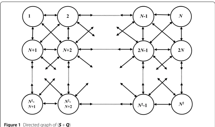
Further, the directed graph of (S+Q) shows that it is an irreducible matrix (see Fig.1). The arrows indicate the pathsi→jfor every nonzero entry of the matrix (S+Q). For any ordered pair of nodesiandj, there exists a direct path (−→i,l1), (

−−→

l1,l2), . . . , ( −→

(12)

(13)

p(j–1)N+k=α1

G(1)_k_,_j2G(3)_k_,_j–G(4)_k_,_j– 2G(1)_x_k_,_j.

For (i= 2(1)N– 1):

M(k–1)N+i= 6B+

h

2[d(k–1)N+i+hp(k–1)N+i] +h

2

2V_i(1)_,_k +V_i(2)_,_k + 43V_i(3)_,_k –V_i(4)_,_k+Oh3, (4.11d)

where

d(k–1)N+i=±

H_i(1)_,_k +H_i(2)_,_k + 23H_i(3)_,_k –H_i(4)_,_k,

p(k–1)N+i=β1

H_i(2)_,_k2H_i(3)_,_k –H_i(4)_,_k– 2H_y(2)_i_,_k,

and, ﬁnally, for ((2≤i≤N– 1), 2≤j≤N– 1):

M(j–1)N+i=h2

V_i(1)_,_j +V_i(2)_,_j + 23V_i(3)_,_j –V_i(4)_,_j +Oh4. (4.11e)

With the help of Eqs. (4.11a)–(4.11e), fork= 1,N, (N– 1)N+ 1 andN2 |dk| ≤(19 + 3α2)G+ (19 + 3β2)H,

|pk| ≤12

α1G2+β1H2+ 3(α1+β1)GH+ 8G(1)+H(2)+ 2G(2)+H(1),

and fork=iand (N– 1)N+i;i= 2(1)N– 1

|dk| ≤10H,

|pk| ≤3β1H2+ 2H(2),

and fork= (j– 1)N+ 1 andjN;j= 2(1)N– 1

|dk| ≤10G,

|pk| ≤3α1G2+ 2G(1).

Hence forh(howsoever small) using(4.11)it is easy to see that

Mk> 9h2V_∗(2); k= 1,N, (N– 1)N+ 1 andN2, (4.12a)

Mk> 19

2 h

2_V(2)

∗ ; k=iand (N– 1)N+i;i= 2(1)N– 1, (4.12b)

Mk> 19

2 h

2_V(2)

∗ ; k= (j– 1)N+ 1 andjN;j= 2(1)N– 1, (4.12c)

M(j–1)N+i≥10h2V∗(2);

i= 2(1)N– 1,j= 2(1)N– 1. (4.12d)

Thus, forh(howsoever small), (S+Q) is monotone. Hence, (S+Q)–1_{exists and (}_S₊_Q₎–1₌

(14)

SinceN_j₌₁2Jl,jMj= 1,l= 1(1)N2, using (4.12a)–(4.12d) withl= 1(1)N2, we obtain

Now, from Eq. (4.10), we obtain

T ≤ JE, (4.14)

Using inequalities (4.13a)–(4.13d) in Eq. (4.15), we get

J ≤ 1651

1710h2_V_∗(2). (4.16)

Finally, with the help of (4.16) for suﬃciently smallh, from (4.14) we obtain

T ≤Oh4. (4.17)

This proves the convergence of the fourth order of the method (4.2) for the elliptic equa-tion (4.1).

5 Method for system of equations

In this section, we extend our method to the system of quasilinear PDEs of the form

A(i)z(_xxi)+C(i)z_yy(i)=k(i)x,y,z(1),z(2), . . . ,z(n),z(1)_x ,z(2)_x , . . . ,z_x(n),z(1)_y ,z(2)_y , . . . ,z(_yn),

i= 1(1)n, (5.1)

where (x,y)∈Γ = (0, 1)×(0, 1),A(i)₌_A(i)₍_x_,_y_{) and}_C(i)₌_C(i)₍_x_,_y_).

The boundary conditions of Dirichlet type are given by

(15)

We assumeZp(i,)qandzp(i,)qto be the exact and approximate values ofz(i)(xp,yq) respectively.

We deﬁne the following approximations:

(16)

ˆˆ diﬀerential equations (5.1) is discretized by

Using the technique discussed in [19], we can derive the fourth order schemes for the system of quasilinear elliptic PDEs.

6 Application to elliptic equations in polar coordinates

In this section, we aim to derive a stable ﬁnite diﬀerence scheme for a class of two-dimensional quasilinear elliptic equations and ensure that the numerical methods devel-oped here retain their order and accuracy everywhere including the region in the vicinity of the singularityx= 0.

Let us consider the elliptic equation of the form

(17)

In this section, we denote

Slm=

∂l+mS

∂xl_∂_ym forl,m= 0, 1, 2, . . . and forS=C,D,G. (6.2) With the help of approximations (2.3a)–(2.11) and using the method (2.12), we obtain the following diﬀerence scheme for Eq. (6.1):

Note that the scheme (6.3) is ofO(h4) for the diﬀerence solution of (6.1). However, the scheme fails when the solution is to be determined atp= 1. We overcome this diﬃculty by modifying the method in such a way that the solutions retain the order and accuracy even in the vicinity of the singularityx= 0.

We consider the following approximations:

Dp±1=Dp±hD10+

Now using the approximations (6.4a)–(6.4c) and neglecting the higher order terms, we get

(18)

Now consider the two dimensional Poisson equation in ther–θplane,

Replacing the variablesx,ybyr,θ, respectively, we get the required difference scheme for the solution of differential equation (6.6) and the coefficients are given by

L1= 1, L2=

Next, we consider the two dimensional Poisson equation in ther–wplane,

zrr+ 1

rzr+zww=G(r,w), 0 <r,w< 1. (6.7)

Replacing the variablesx,ybyr,w, respectively, we get the required difference scheme for the solution of the differential equation (6.7) and the coefficients are given by

L1= 1, L2= 1, L3= 0, L4=

Note that the scheme (6.3) along with the approximations (6.4a)–(6.4c) are ofO(h4_{) and}

free from the terms 1/(p±1) and 1/(q±1), hence it is very easily solved forp,q= 1, 2, . . . ,N

in the region 0 <r,θ< 1 and 0 <r,w< 1. In a similar manner, we can discuss the numerical schemes for nonlinear elliptic equations in polar coordinates.

7 Application to nonlinear bi- and triharmonic problems

7.1 Nonlinear biharmonic equation

We consider the 2D nonlinear biharmonic elliptic partial diﬀerential equation with a forc-ing function of the form

∇4_z₍_x_,_y_{) =}_f_x_,_y_,_z_,_∇2_z_,_z

The boundary conditions of second kindzand (∂2z/∂n2_{) are prescribed on the boundary.}

(19)

axes and the values ofzare exactly known on the boundary, this implies that the successive tangential partial derivatives ofzare known exactly on the boundary. For example, on the liney= 0, the values ofz(x, 0) andzyy(x, 0) are known, i.e. the values ofzx(x, 0),zxx(x, 0), etc. are known on the liney= 0. This implies the values ofz(x, 0) and∇2_z₍_x_{, 0)}_≡_z

xx(x, 0) +

zyy(x, 0) are known on the liney= 0. Similarly, the values ofzand∇2zare known on all sides of the square region.

Let us denote∇2_z₌_v_{. Then we can rewrite Eq. (7.1) in a coupled manner as}

∇2_z₌_v₍_x_,_y_), ₍_x_,_y₎_∈_Γ_, _(7.2a)

∇2_v₌_f₍_x_,_y_,_z_,_v_,_z

x,vx,zy,vy), (x,y)∈Γ. (7.2b)

In this case, the values ofzandvare exactly known on the boundary ofΓ.

Applying the method (5.12) to the system of equations (7.2a)–(7.2b), a numerical method of order four for the solution of the biharmonic equation (7.1) can be written as

δ2_x+δ2_y+1 6

δ2_xδ_y2Zp,q

=h2Vp,qexp

Vp+1,q+Vp–1,q+Vp,q+1+Vp,q–1– 4Vp,q 12Vp,q

+Oh6,

1≤p,q≤N, (7.3a)

δ2_x+δ2_y+1 6

δ2_xδ_y2Vp,q

=h2Fp,qexp

Fp+1,q+Fp–1,q+Fp,q+1+Fp,q–1– 4Fˆˆp,q 12Fp,q

+Oh6,

1≤p,q≤N, (7.3b)

where

Fp±1,q=f(xp±1,yq,zp±1,q,vp±1,q,z¯xp±1,q,¯vxp±1,q,z¯yp±1,q,v¯yp±1,q), (7.4a)

Fp,q±1=f(xp,yq±1,zp,q±1,vp,q±1,z¯xp,q±1,¯vxp,q±1,z¯yp,q±1,v¯yp,q±1), (7.4b) ¯¯

Fp,q=f(xp,yq,zp,q,vp,q,z¯¯xp,q,¯¯vxp,q,z¯¯yp,q,v¯¯yp,q), (7.4c) ˆˆ

Fp,q=f(xp,yq,zp,q,vp,q,zˆˆxp,q,ˆˆvxp,q,zˆˆyp,q,vˆˆyp,q). (7.4d)

The approximations associated with (7.4a)–(7.4d) are already deﬁned in Sect.5.

7.2 Nonlinear triharmonic equation

Next we consider the nonlinear triharmonic equation with a forcing function of the form

∇6_z₍_x_,_y_{) =}_g_x_,_y_,_z_,_∇2_z_,_∇4_z_,_z

x,∇2zx,∇4zx,zy,∇2zy,∇4zy

, Γ : 0 <x,y< 1. (7.5)

(20)

For Eq. (7.5), the boundary values ofz,zyy,zyyyyare prescribed on the liney= 0,y= 1; and the boundary values ofz,zxx,zxxxxare prescribed on the linex= 0,x= 1. As discussed in the biharmonic case, the values ofz,∇2_z_and_∇4_z_{are known on all sides of the square}

regionΓ.

Let∇2_z₌_v_and_∇2_v₌_w_{. Then we rewrite Eq. (7.5) in a split form as}

∇2_z₌_v₍_x_,_y_), ₍_x_,_y₎_∈_Γ_, _(7.6a)

∇2_v₌_w₍_x_,_y_), ₍_x_,_y₎_∈_Γ_, _(7.6b)

∇2_w₌_g₍_x_,_y_,_z_,_v_,_w_,_z

x,vx,wx,zy,vy,wy), (x,y)∈Γ. (7.6c) Applying the method (5.12) to the system of equations (7.6a)–(7.6c), a numerical method of order four for the solution of triharmonic equation (7.5) can be written as

δ2_x+δ2_y+1 6

δ2_xδ_y2Zp,q

=h2Vp,qexp

Vp+1,q+Vp–1,q+Vp,q+1+Vp,q–1– 4Vp,q 12Vp,q

+Oh6,

1≤p,q≤N, (7.7a)

δ2_x+δ2_y+1 6

δ2_xδ_y2Vp,q

=h2Wp,qexp

Wp+1,q+Wp–1,q+Wp,q+1+Wp,q–1– 4Wp,q 12Wp,q

+Oh6,

1≤p,q≤N, (7.7b)

δ2_x+δ2_y+1 6

δ2_xδ_y2Wp,q

=h2Gp,qexp

Gp+1,q+Gp–1,q+Gp,q+1+Gp,q–1– 4Gp,q 12Gp,q

+Oh6,

1≤p,q≤N, (7.7c)

where

Gp±1,q=g(xp±1,yq,zp±1,q,vp±1,q,wp±1,q,¯zxp±1,q,v¯xp±1,q, ¯

wxp±1,q,z¯yp±1,q,v¯yp±1,q,w¯yp±1,q), (7.8a)

Gp,q±1=g(xp,yq±1,zp,q±1,vp,q±1,wp,q±1,¯zxp,q±1,v¯xp,q±1, ¯

wxp,q±1,z¯yp,q±1,v¯yp,q±1,w¯yp,q±1), (7.8b) ¯¯

Gp,q=f(xp,yq,zp,q,vp,q,wp,q,z¯¯xp,q,¯¯vxp,q,w¯¯xp,q,z¯¯yp,q,v¯¯yp,q,w¯¯yp,q), (7.8c) ˆˆ

Gp,q=g(xp,yq,zp,q,vp,q,wp,qzˆˆxp,q,vˆˆxp,q,wˆˆxp,q,zˆˆyp,q,vˆˆyp,q,wˆˆyp,q). (7.8d)

The approximations associated with (7.8a)–(7.8d) are already deﬁned in Sect.5.

(21)

equations (7.1), (7.5). A direct solution of these linear systems is impractical because of the large size of the coeﬃcient matrix and enormous storage requirements even for moderate values of the grid size. Classical block iterative methods such as the Gauss–Seidel and successive over relaxation methods are attractive for their low storage requirements as long as convergence is guaranteed.

8 Numerical illustrations

We implement the proposed method on ten benchmark problems of 2D elliptic equations. The exact solution of each problem is given. The right hand side function and Dirichlet boundary conditions are determined from the exact solution in each problem. The sys-tem of linear diﬀerence equations are solved using the Gauss–Seidel iteration method and that of nonlinear diﬀerence equations by the Newton–Raphson iteration method [36,37]. The iterations are terminated once the absolute error tolerance≤10–12_{is reached and the}

initial guess made in each case is z = 0. All computations were performed using MATLAB codes.

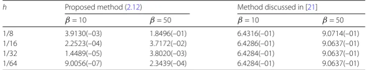
Problem 8.1(Convection–diﬀusion equation)

zxx+zyy=βzx, 0 <x,y< 1. (8.1)

The exact solution is given by z(x,y) =eβx/2sin(πy)

sinh(σ)[2e

–β/2_sinh₍_σ_x_{) +}_sinh₍_σ_{(1 –}_x_))],_σ ₌

π2₊β2 4.

The maximum absolute errors (MAEs) inzare listed in Table1. Figures2(a) and (b) give the plots of the exact and numerical solutions forh= 1/64 andβ= 50.

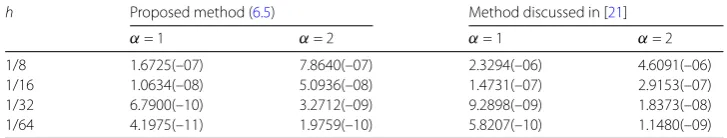
Problem 8.2(Poisson’s equation inr–θplane)

zrr+

α

rzr+

1

r2zθ θ=G(r,θ), 0 <r,θ< 1. (8.2)

The exact solution isz(r,θ) =r2cos(π θ). The MAEs inzare listed in Table2forα= 1 and 2. Figures3(a) and (b) give the plots of the exact and numerical solutions forh= 1/32 and

α= 2.

Problem 8.3(Poisson’s equation inr–wplane)

zrr+

α

rzr+zww=G(r,w), 0 <r,w< 1. (8.3)

The exact solution isz(r,w) =coshrcoshw. The MAEs inzare listed in Table3forα= 1 and 2. Figures4(a) and (b) give the plots of the exact and numerical solutions forh= 1/64 andα= 2.

Table 1 Problem8.1: The maximum absolute errors

h Proposed method (2.12) Method discussed in [21]

β= 10 β= 50 β= 10 β= 50

1/8 3.9130(–03) 1.8496(–01) 6.4316(–01) 9.0714(–01)

1/16 2.2523(–04) 3.7172(–02) 6.4286(–01) 9.0637(–01)

1/32 1.4489(–05) 3.8020(–03) 6.4284(–01) 9.0637(–01)

(22)

(a)

(b)

Figure 2(a) Exact solution of Problem8.1forh= 1/64 andβ= 50. (b) Numerical solution of Problem8.1for h= 1/64 andβ= 50

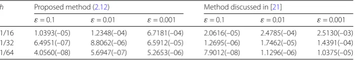
Problem 8.4(Burgers’ equation)

ε(zxx+zyy) =z(zx+zy) +g(x,y), 0 <x,y< 1. (8.4)

The exact solution is z(x,y) =ex_sin₍πy

2 ). The MAEs inzare listed in Table 4forε=

(23)

α= 1 α= 2 α= 1 α= 2

1/8 1.6725(–07) 7.8640(–07) 2.3294(–06) 4.6091(–06)

1/16 1.0634(–08) 5.0936(–08) 1.4731(–07) 2.9153(–07)

1/32 6.7900(–10) 3.2712(–09) 9.2898(–09) 1.8373(–08)

1/64 4.1975(–11) 1.9759(–10) 5.8207(–10) 1.1480(–09)

(a)

(b)

(24)

α= 1 α= 2 α= 1 α= 2

1/8 8.7756(–07) 4.5043(–07) 1.6604(–06) 2.8030(–06)

1/16 4.1258(–08) 3.4516(–08) 1.0530(–07) 1.7649(–07)

1/32 1.8296(–09) 2.4751(–09) 6.6915(–09) 1.1082(–08)

1/64 1.1482(–10) 1.4936(–10) 4.2259(–10) 6.9292(–10)

(a)

(b)

(25)

ε= 0.1 ε= 0.01 ε= 0.001 ε= 0.1 ε= 0.01 ε= 0.001 1/16 1.0393(–05) 1.2348(–04) 6.7181(–04) 2.0616(–05) 2.4785(–04) 2.5130(–03) 1/32 6.4951(–07) 8.8062(–06) 6.5912(–05) 1.2695(–06) 1.7462(–05) 1.4391(–04) 1/64 4.0560(–08) 5.6947(–07) 5.2653(–06) 7.9012(–08) 1.1296(–06) 1.0375(–05)

(a)

(b)

(26)

Re= 10 Re= 102 Re= 10 Re= 102

1/16 z 1.2914(–06) 1.0250(–05) 3.8170(–05) 7.9117(–04) v 1.5074(–06) 4.9247(–05) 2.0205(–05) 8.1179(–04)

1/32 z 8.1723(–08) 5.7969(–06) 2.4148(–06) 4.4070(–05) v 9.2739(–08) 3.0772(–06) 1.2680(–06) 4.6982(–05)

1/64 z 5.1144(–09) 3.5421(–07) 1.5149(–07) 2.6562(–06) v 5.7879(–09) 1.9343(–07) 7.9504(–08) 3.0175(–06)

Problem 8.5(2D steady-state Navier–Stokes model equations in rectangular coordinates)

1 Re

(zxx+zyy) =zzx+vzy+f(x,y), 0 <x,y< 1, (8.5a) 1

Re

(vxx+vyy) =zvx+vvy+g(x,y), 0 <x,y< 1. (8.5b)

The exact solutions arez(x,y) =sin(πx)sin(πy),v(x,y) =cos(πx)cos(πy).

The MAEs inz,vare tabulated in Table5for various values of the Reynolds numberRe. Figures6(a) and (b) give the plots of the exact and numerical solutions ofzand Figs.6(c) and (d) give the plots of the exact and numerical solutions ofvforh= 1/64,Re= 10.

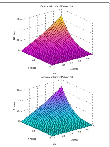
Problem 8.6(2D steady-state Navier–Stokes model equations in cylindrical polar

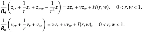
coor-dinates inr–wplane) 1

Re

zrr+ 1

rzr+zww–

1

r2z

=zzr+vzw+H(r,w), 0 <r,w< 1, (8.6a) 1

Re

vrr+ 1

rvr+vzz

=zvr+vvw+I(r,w), 0 <r,w< 1. (8.6b)

The exact solutions are given byz(r,w) =r3_sinh_w_,_v₍_r_,_w_{) = –4}_r2_cosh_w_{. The MAEs in}_z_,_v

are listed in Table6for various valuesRe. Figures7(a) and (b) give the plots of the exact and numerical solutions ofz, and Figs.7(c) and (d) give the plot of the exact and numerical solutions ofvforh= 1/32 andRe= 10.

Problem 8.7(Nonlinear elliptic equation)

1 +x2zxx+

1 +y2zyy=αz(zx+zy) +f(x,y), 0 <x,y< 1. (8.7)

The exact solution isz(x,y) =ex_cos₍_π_y_{). The MAEs in}_z_{are tabulated in Table}₇_{for various} values ofα. Figures8(a) and (b) give the plot of the exact and numerical solutions ofzfor the values ofh= 1/64 andα= 1.

Problem 8.8(Quasilinear elliptic equation)

zxx+

(27)

(a)

(b)

Figure 6(a) Exact solution of Problem8.5forz(x,y) forh= 1/64 and Re = 10. (b) Numerical solution of Problem8.5forz(x,y) forh= 1/64 and Re = 10. (c) Exact solution of Problem8.5forv(x,y) forh= 1/64 and Re = 10. (d) Numerical solution of Problem8.5forv(x,y) forh= 1/64 and Re = 10

The exact solution isz(x,y) =excos(πy). The MAEs inzare tabulated in Table8for various values ofα. Figures9(a) and (b) give the plots of the exact and numerical solutions ofzfor

h= 1/64 andα= 1.

Problem 8.9(Nonlinear biharmonic equation)

∇4_z₌_α_z_z

x+zy+∇2zx+∇2zy

(28)

(c)

(d)

Figure 6Continued

The exact solution isz(x,y) =sin(πx)cos(πy). The MAEs inzare tabulated in Table9for various values ofα. Figures10(a) and (b) give the plots of the exact and numerical solutions

ofzforh= 1/64 andα= 1.

Problem 8.10(Nonlinear triharmonic Equation)

∇6_z₌_α_z_z

x+zy+∇2zx+∇2zy+∇4zx+∇4zy

(29)

Re= 10 Re= 102 Re= 10 Re= 102

1/8 z 2.4506(–03) 5.8523(–03) 6.6056(–03) 7.5996(–03)

v 1.2759(–03) 4.2671(–03) 9.8564(–03) 2.0399(–02)

1/16 z 1.5568(–04) 3.7093(–04) 8.6235(–04) 1.9389(–03) v 8.4150(–05) 2.6707(–04) 8.9744(–04) 3.6708(–03)

1/32 z 9.8510(–06) 2.3438(–05) 6.3020(–05) 3.8183(–04) v 5.2923(–06) 1.6697(–05) 5.7202(–05) 4.9547(–04)

(a)

(b)

(30)

(c)

(d)

Figure 7Continued

α= 10 α= 25 α= 10 α= 25

1/16 3.8618(–05) 2.6193(–04) 1.4642(–04) 4.8477(–04)

1/32 2.4173(–06) 1.4481(–05) 9.1279(–06) 2.9675(–05)

1/64 1.5114(–07) 8.7080(–07) 5.6914(–07) 1.8430(–06)

(31)

(a)

(b)

Figure 8(a) Exact solution of Problem8.7forh= 1/64 andα= 1. (b) Numerical solution of Problem8.7for h= 1/64 andα= 1

α= 1 α= 5 α= 10 α= 1 α= 5 α= 10

1/16 2.2420(–06) 2.8725(–06) 2.6025(–05) 2.5631(–05) 3.8351(–05) 3.0062(–04) 1/32 1.4784(–07) 1.9884(–07) 1.6322(–06) 1.7057(–06) 2.2772(–06) 1.8240(–05) 1/64 9.8422(–09) 1.2414(–08) 1.0205(–07) 1.0974(–07) 1.4068(–07) 1.1322(–06)

9 Conclusions

(32)

dif-(a)

(b)

Figure 9(a) Exact solution of Problem8.8forh= 1/32 and Re = 10. (b) Numerical solution of Problem8.8for h= 1/64 andα= 1

h Proposed method (7.3a)–(7.3b) Method discussed in [25]

α= 1 α= 5 α= 10 α= 1 α= 5 α= 10

1/16 2.5145(–06) 5.2636(–06) 9.8678(–06) 7.4745(–05) 5.5647(–05) 3.6038(–05) 1/32 1.5722(–07) 3.3169(–07) 6.1875(–07) 5.1113(–06) 3.6668(–06) 2.4504(–06) 1/64 9.7708(–09) 2.0628(–08) 3.9183(–08) 3.3505(–07) 2.3238(–07) 1.5557(–07)

(33)

prob-(a)

(b)

Figure 10 (a) Exact solution of Problem8.9forh= 1/32 andα= 10. (b) Numerical solution of Problem8.9for h= 1/32 andα= 10

h Proposed method (7.7a)–(7.7c) Method discussed in [27]

α= 1 α= 5 α= 10 α= 1 α= 5 α= 10

1/16 2.3858(–06) 3.2640(–06) 4.4844(–06) 8.6722(–05) 6.5269(–05) 4.2669(–05) 1/32 1.4986(–07) 2.0592(–07) 2.8234(–07) 5.1941(–06) 4.1014(–06) 2.6692(–06) 1/64 9.1825(–09) 1.2267(–08) 1.6584(–08) 3.1737(–07) 2.5784(–07) 1.6686(–07)

(34)

(a)

(b)

Figure 11 (a) Exact solution of Problem8.10forh= 1/64 andα= 10. (b) Numerical solution of Problem8.10

forh= 1/64 andα= 10

and compared with the results of existing methods. The theoretical rate of convergence was corroborated by the experimentally observed rate of convergence using the formula

ρ=log(eh1/eh2)/log(h1/h2), whereeh1 andeh2 are the maximum absolute errors for two mesh sizesh1andh2respectively. Computational results exhibit that the proposed

(35)

Acknowledgements

The authors thank the reviewers for their valuable suggestions, which substantially improved the quality of the paper.

Funding

This work is supported by Maitreyi College, University of Delhi.

Competing interests

The authors declare that they have no competing interests.

Authors’ contributions

All authors drafted the manuscript, and they read and approved the ﬁnal version.

Author details

1_{Department of Applied Mathematics, South Asian University, New Delhi, India.}2_{Department of Mathematics, Faculty of}

Natural Sciences, Jamia Millia Islamia University, New Delhi, India.3_{Present address:}_{Department of Mathematics, Maitreyi}

College, University of Delhi, Delhi, India.

Publisher’s Note

Springer Nature remains neutral with regard to jurisdictional claims in published maps and institutional aﬃliations.

Received: 19 September 2018 Accepted: 15 January 2019 References

1. Jain, M.K., Jain, R.K., Mohanty, R.K.: Fourth order difference methods for the system of 2D nonlinear elliptic partial differential equations. Numer. Methods Partial Differ. Equ.7, 227–244 (1991)

2. Jain, M.K., Jain, R.K., Mohanty, R.K.: A fourth order difference method for elliptic equations with nonlinear first derivative terms. Numer. Methods Partial Differ. Equ.5, 87–95 (1989)

3. Li, M., Tang, T., Fornberg, B.: A compact fourth-order ﬁnite diﬀerence scheme for the steady state incompressible Navier–Stokes equations. Int. J. Numer. Methods Fluids20, 1137–1151 (1995)

4. Erturk, E., Gökcöl, C.: Fourth-order compact formulation of Navier–Stokes equations and driven cavity ﬂow at high Reynolds numbers. Int. J. Numer. Methods Fluids50, 421–436 (2006)

5. Liu, J., Wang, C.: A fourth order numerical method for the primitive equations formulated in mean vorticity. Commun. Comput. Phys.4, 26–55 (2008)

6. Ito, K., Qiao, Z.: A high order compact MAC ﬁnite diﬀerence scheme for the Stokes equations: augmented variable approach. J. Comput. Phys.227, 8177–8190 (2008)

7. Spotz, W.F., Carey, G.F.: High order compact scheme for the steady stream function vorticity equations. Int. J. Numer. Methods Eng.38, 3497–3512 (1995)

8. Carey, G.F.: Computational Grids: Generation, Adaption and Solution Strategies. Taylor & Francis, Washington (1997) 9. Yavneh, I.: Analysis of a fourth-order compact scheme for convection diﬀusion. J. Comput. Phys.133, 361–364 (1997) 10. Zhang, J.: On convergence of iterative methods for a fourth-order discretization scheme. Appl. Math. Lett.10, 49–55

(1997)

11. Birkhoﬀ, G., Lynch, R.E.: The Numerical Solution of Elliptic Problems. SIAM, Philadelphia (1984)

12. Mohanty, R.K.: Fourth order finite difference methods for the system of 2D nonlinear elliptic equations with variable coefficients. Int. J. Comput. Math.46, 195–206 (1992)

13. Böhmer, K.: On ﬁnite element methods for fully nonlinear elliptic equations of second order. SIAM J. Numer. Anal. 46(3), 1212–1249 (2008)

14. Feng, X., Neilan, M.: Vanishing moment method and moment solution for fully nonlinear second order partial diﬀerential equations. J. Sci. Comput.38, 78–98 (2009)

15. Böhmer, K.: Numerical Methods for Nonlinear Elliptic Diﬀerential Equations: A Synopsis. Oxford University Press, Oxford (2010)

16. Jain, M.K., Jain, R.K., Krishna, M.: Fourth order diﬀerence method for quasi-linear Poisson equation in cylindrical symmetry. Commun. Numer. Methods Eng.10, 291–296 (1994)

17. Ananthakrishnaiah, U., Saldanha, G.: A fourth order finite difference scheme for two-dimensional non-linear elliptic partial differential equations. Numer. Methods Partial Differ. Equ.11, 33–40 (1995)

18. Mohanty, R.K.: Orderh4_{diﬀerence methods for a class of singular two-space dimensional elliptic boundary value}

problems. J. Comput. Appl. Math.81, 229–247 (1997)

19. Mohanty, R.K., Dey, S.: A new ﬁnite diﬀerence discretization of order four for (∂u/∂n) for two-dimensional quasi-linear elliptic boundary value problems. Int. J. Comput. Math.76, 505–576 (2001)

20. Mohanty, R.K., Singh, S.: A new fourth order discretization for singularly perturbed two dimensional non-linear elliptic boundary value problems. Appl. Math. Comput.175, 1400–1414 (2006)

21. Mohanty, R.K., Setia, N.: A new compact high order off-step discretization for the system of 2D quasi-linear elliptic partial differential equations. Adv. Differ. Equ.2013, 223 (2013)

22. Zhang, J.: On convergence and performance of iterative methods with fourth order compact schemes. Numer. Methods Partial Diﬀer. Equ.14, 263–280 (1998)

23. Saldanha, G.: Technical note: a fourth order finite difference scheme for a system of 2D nonlinear elliptic partial differential equations. Numer. Methods Partial Differ. Equ.17, 43–53 (2001)

24. Arabshahi, S.M.M., Dehghan, M.: Preconditioned techniques for solving large sparse linear systems arising from the discretization of the elliptic partial diﬀerential equations. Appl. Math. Comput.188, 1371–1388 (2007)

(36)

26. Mohanty, R.K.: Single cell compact finite difference discretizations of order two and four for multi-dimensional triharmonic problems. Numer. Methods Partial Differ. Equ.26, 1420–1426 (2010)

27. Mohanty, R.K., Jain, M.K., Mishra, B.N.: A compact discretization ofO(h4_{) for two-dimensional non-linear triharmonic}

equations. Phys. Scr.84, 025002 (2011)

28. Mohanty, R.K., Jain, M.K., Mishra, B.N.: A novel numerical method ofO(h4_{) for three-dimensional non-linear}

triharmonic equations. Commun. Comput. Phys.12, 1417–1433 (2012)

29. Khattar, D., Singh, S., Mohanty, R.K.: A new coupled approach high accuracy numerical method for the solution of 3D non-linear biharmonic equations. Appl. Math. Comput.215, 3036–3044 (2009)

30. Singh, S., Khattar, D., Mohanty, R.K.: A new coupled approach high accuracy numerical method for the solution of 2D non-linear biharmonic equations. Neural Parallel Sci. Comput.17, 239–256 (2009)

31. Singh, S., Singh, S., Mohanty, R.K.: A new high accuracy oﬀ-step discretization for the solution of 2D non-linear triharmonic equations. East Asian J. Appl. Math.03, 228–246 (2013)

32. Gautschi, W.: Numerical integration of ordinary diﬀerential equations based on trigonometric polynomials. Numer. Math.3, 381–397 (1961)

33. Lyche, T.: Chebyshevian multistep methods for ordinary diﬀerential equations. Numer. Math.19, 65–75 (1972) 34. Varga, R.S.: Matrix Iterative Analysis. Springer, New York (2000)

35. Hageman, L.A., Young, D.M.: Applied Iterative Methods. Dover, New York (2004)