Rupture proce
ss
of the 2007 Notohanto earthquake by u
s
ing an i
s
ochrone
s
back-projection method and K-NET/KiK-net data
Nelson Pulido, Shin Aoi, and Hiroyuki Fujiwara
National Research Institute for Earth Science and Disaster Prevention, Japan
(Received June 30, 2007; Revised February 27, 2008; Accepted March 24, 2008; Online published November 7, 2008)
We estimated the source process of the 2007/3/25 Notohanto earthquake using a new method for source imaging based on an “isochrones-backprojection” of observed seismograms in the source region (IBM). The IBM differs fromconventional earthquake sourcemodeling approaches in that no inversion procedures are required. The idea of IBM is to directly back-project amplitudes of seismogramenvelopes around the source into a space image of the earthquake rupture. Themethod requires the calculation of isochrones times at every station used for source imaging, for a set of grids points distributed within the source fault plane. Total grid “brightness” is calculated by adding all observed waveformenvelope amplitudes at every station, for every isochrone line crossing the grid, in order to produce an image of the total fault plane brightness distribution. Our source imaging results of the Notohanto earthquake show two large brightness regions; the first region is located 10 kmabove the hypocenter, and the second region is located at the bottomof the northern end of the fault plane. These regions approximately correspond to large slip areas obtained by a conventional inversion approach. Ourmethod has the capability to quicklymap asperities of large earthquakes using observed strongmotion data.
Key words:Source process, array imaging, high frequency, Notohanto earthquake.
1.
Introduction
The 2007 Notohanto earthquake (Mw =6.7, 2007/3/25,
JT 09:41:57.9) was located by the Japan Meteorological Agency (JMA) at a latitude of 37.220, longitude of 136.685 and depth of 11 km. According to the National Research Institute for Earth Science and Disaster Prevention broad-band network (F-NET, NIED), the earthquake had a reverse
mechanismwith a highly oblique slip direction (strike 58◦, dip 66◦and rake 132◦). The Notohanto earthquake recorded JMA instrumental intensities up to 6 (upper), and ground accelerations and velocities reached values of 850 gals and 100 kines respectively, at NIED, K-NET sites. The earth-quake ground shaking induced amassive damage to houses and roads and triggeredmany rock and embankment fail-ures around the source (Hamadaet al., 2007).
Standard methodologies for calculation of the earth-quakes source process are based on inversion procedures which require the calculation of complete source-stations Greens functions (i.e. Hartzell and Heaton, 1983; Sekiguchi
et al., 2002; and others). Alternative procedures have been developed in order to directly retrieve an image of the rup-ture process fromhigh-frequency seismograms around the source (Spudich and Cranswick, 1984; Ellsworth, 1992; Ishiiet al., 2005; Fletcheret al., 2006; Kao and Shan, 2007; Allmann and Shearer, 2007). Other procedures have im -plemented the concept of isochrones introduced by Bernard and Madariaga (1984) and Spudich and Frazer (1984) to ob-tain amap of the fault slip fromthe back-projection of
near-Copyright cThe Society of Geomagnetismand Earth, Planetary and Space Sci-ences (SGEPSS); The Seismological Society of Japan; The Volcanological Society of Japan; The Geodetic Society of Japan; The Japanese Society for Planetary Sci-ences; TERRAPUB.
source seismograms (Iwata and Irikura, 1989; Festa, 2004; Festa and Zollo, 2006). Festa and Zollo (2006) applied this
method to investigate the source process of the 2000 Tottori earthquake fromnear-source low frequency seismograms.
In this study we extend the methodology of Festa and Zollo (2006) by incorporating the use of high-frequency (HF) seismograms for imaging the source rupture. To fa-cilitate the use of HF waveforms we calculate envelopes of velocity seismograms to image the fault plane brightness by constraining the fault rupture to a constant value. We apply the isochrones back-projectionmethod (IBM) to ob-tain an image of the large brightness regions across the fault plane of the 2007 Notohanto earthquake. We found that our
methodology is capable of quicklymap asperities of large tomoderate earthquakes by using strongmotion waveforms and is able to provide stable estimates of the fault rupture velocity.
2.
The I
s
ochrone
s
Back-projection Method
The main idea of the IBM is to directly back-project amplitudes of seismograms envelopes around the source into a space image of the earthquake rupture. Themethod requires the calculation of theoretical travel times between a set of grid points distributed across the fault plane and every station, which are adjusted by a station correction factor, for a 1D velocity model. Next we calculate the rupture time of every grid within the fault plane by assuming some arbitrary constant rupture velocity value, and obtain the isochrones times for every station. We select waveforms that have clear P- and S-wavelets, which means stations located approximately between 40 km and 100 km from
the epicenter. We extract P-wave windows between the
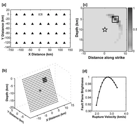
Fig. 1. (a) Station distribution used for the resolution test. The stations are uniformly spaced at 40 km, and the source is located at the origin. (b) Fault plane used for the source imaging. The plane is dipping 66◦ down-wards theY-axis. The black dots represent the asperity location used to calculate the synthetic seismograms. (c) Results of the IBM source imaging (normalized fault brightness) for a rupture velocity value of 2.5 km/s (color scale). The assumed asperity is enclosed by a black square. (d) Rupture velocity vs normalized total fault plane brightness.
origin time of the earthquake and the theoretical arrival of the S-wave, taper 1 s of the waveforms towards the end, and apply a band-pass filter between 1 and 30 Hz. Velocity envelopes (V) are calculated using the root-mean-square of the original seismograms and their Hilbert transform(H),
V[v(t)]=(v(t)2+H2[v(t)])2 (1)
where v(t) are the velocity waveforms. The total grid brightness (Eg) is calculated by adding averaged envelope
amplitudes, for a window centered at the grid isochrone time for all stations,
Eg=
whereAis the envelope value,Nis the total number of sta-tions,W is the envelope averaging window half width,tgi is
the travel time between gridg and stationi,tgrupis the grid
rupture time,t is the sampling time,ciis the station
cor-rection time for thei station, and Rgi is the source-station
ray length, intended as a correction for geometrical spread-ing. We apply appropriate data weighting factorswi, which
can be representative of the quality of the data. In this case, we assign the weights a value proportional to the station epicentral distance, in order to tapermigration artifacts pro-duced by stations towards the perimeter of the array
(All-mann and Shearer, 2007). The calculation of grid bright-ness in Eq. (2), is similar to the envelope averaging proce-dure of Kao and Shan (2007), but introduces the concept of isochrones times to constraint the fault rupture. We calcu-late the total brightness for all grids across the fault plane and normalize the values by themaximumgrid brightness. In this way we obtain the brightness distribution across the
slip obtained fromconventional inversion proceduresmay be useful to determine a scaling relationship between grid brightness and fault slip. Thismay be a subject for future research.
3.
Source Image Po
s
t-proce
ss
ing
The source images obtained by the IBM are usually characterized by a defocusing along the isochrones lines,
mainly arising fromthe assumption of a uniform bright-ness distribution along the isochrones as well as poor az-imuth station coverage, as pointed out by Festa and Zollo (2006). To remove this effect, we apply the “restarting” procedure described in Festa and Zollo (2006) to the back-projected images of brightness. This procedure consists of using the result of the first back-projected images as a pri-ori information for a new back-projection. Festa and Zollo (2006) found that the application of the restarting itera-tive procedure to back-projected images of the 2000 Tot-tori, Japan earthquake lead to a significant improvement of the observed-synthetic data fit. The number of iterations will depend on an observation-synthetic fit criterion. In our
methodology we do not calculate forward envelopes in or-der to allow for a quickmapping of the source brightness, and therefore, we adopt an iteration value that allows us to sufficiently reduce the defocusing effect. On the other hand, the introduction of a specific source-station ray length in Eq. (2), intended as a simple correction for geometrical spreading, also contributes to reducing the defocusing effect along the isochrones.
4.
Re
s
olution Te
s
t
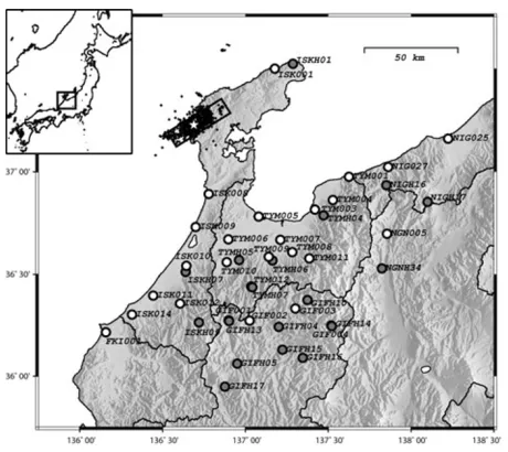
neg-Fig. 2. K-NET and KiK-net stations used for the source imaging of the 2007 Notohanto earthquake (Mw6.7), depicted as white and gray
circles, respectively. The crosses represent the first 24 h of aftershocks withmagnitude larger than 2. A white star depicts the JMA epicenter of themainshock, and a black rectangle the fault planemodel used for source imaging.
ative adjacent triangles with a total duration of 0.4 s, which would approximately correspond to the far-field velocity ra-diation of a ramp dislocation at the source. We norm al-ize the pulse by its maximumamplitude and divide it by the epicentral distance as an approximation for geom etri-cal spreading. The arrival time of the pulse at every station is specified by the isochrone time, which is calculated for a uniformrupture velocity and for a half-space with a P -wave velocity of 6 km/s. Total groundmotion at every sta-tion is calculated by adding the contribusta-tion fromall point sources. To simulate realistic conditions we incorporate a randomsite amplification to each station and add a 20% of normal noise.
We apply themethodology for source imaging described in Sections 2 and 3, using the synthetic waveforms and the grid geometry in Fig. 1(b). The results of source imaging are shown in Fig. 1(c). We can observe that the IBM is able to illuminate the assumed asperity location, depicted as a black rectangle in Fig. 1(c). We also performed the IBM source imaging for a randomdistribution of stations cover-ing a similar area than the configuration in Fig. 1(a), and found that the asperity location was imaged unequivocally. Although the asperity location is correctly identified in all cases, we have found that the imaged source has an elon-gated Kernel along the imaged asperity. This featuremay result frompoor station coverage as well as the assumption of an instantaneous slip in the isochronesmethod (Spudich and Frazer, 1984). On the other hand, we have found that using a distribution of stations located closer that 40 km
around the source area, for various spacing values, always lead to a wrong imaging of the asperity location. This result can be useful for the station selection process for the source imaging of actual earthquakes.
We repeated the source imaging for the fault and station configuration in Fig. 1, but assuming different values of
Fig. 3. Velocitymodel for the Atotsugawa fault region (Ito and Wada, 2002), depicted as a continous black line with dots. Themultilayered
model show as a gray line is used for the calculation of travel times for the source imaging of the Notohanto earthquake.
fault rupture velocity. We found that the total fault plane brightness, obtained by adding the brightness of all grids across the fault plane, have a maximumfor a value close to the rupture velocity used for the synthetic waveforms calculation (Fig. 1(d)). This result may be explained by the fact that when no radiation is occurring at the imaged grid, the summation of envelopes at all stations will not be coherent. In other words, the overall summation of envelopes will reach amaximumfor a rupture velocity that approaches the actual value.
5.
Notohanto Earthquake Data
We used waveforms of the Notohanto earthquake recorded at 44 NIED strong motion stations (26 K-NET, and 18 KiK-net) for the source imaging of the earthquake (Fig. 2). We selected records with distinct P- and S -wavelets, which corresponded in general to stations with epicentral distances ranging from40 to 150 km. In order to calculate travel times, we set amesh of point sources uni-formly spaced at 2 km, across a plane with dip and strike an-gles corresponding to the F-NET solution (strike N58◦, dip 66◦), intersecting the JMA hypocenter solution. The shal-lower row of point sources is located at a depth of 1.89 km, and the grid-mesh covers a rectangular area of 22 kmalong dip and 34 kmalong strike, as shown in Fig. 2. We calcu-lated all travel times between grids and stations using a ve-locitymodel developed for the Atotsugawa fault region (Ito and Wada, 2002) (Figs. 3 and 4). For simplicity, the original velocity was parameterized as amultilayeredmodel with no gradients (Fig. 3). All grid travel times were adjusted by a station correction factor, obtained by calculating the dif-ference between observed and calculated travel times at all stations for anM5.3 aftershock (2007/03/25, 18:11:00).
6.
Re
s
ult
s
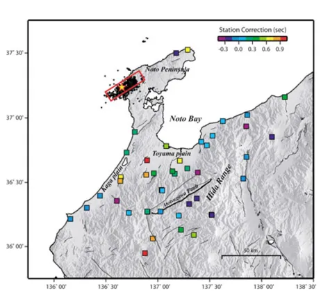
6.1 Stationscorrections
Fig. 4. Station corrections obtained as the difference between calculated and observed travel times for an M5.3 aftershock of the Notohanto earthquake (colored squares). The crosses represent the first 24 h of aftershocks withmagnitude larger than 2. A star depicts the JMA epicenter of themainshock and a red rectangle the fault planemodel used for imaging. Thin black lines represent faults in the region.
Fig. 5. Normalized fault plane brightness distribution obtained by the Isochrones Back-Projection Method (in a color scale). A slipmodel of the Notohanto earthquake obtained by an inversion of near-source strong groundmotions is overlapped as black contour lines (everym e-ter), and gray arrows, with amaximumslip of 4.3m(Aoi and Sekiguchi, 2007). A red star depicts the rupture starting point. The fault configura-tion and grid spacing (2 km) is the same for bothmodels.
are expected, and smaller towards stations within the Hida range (Fig. 4).
6.2 Source image of the Notohanto earthquake
We applied the procedures outlined in the previous sec-tions to obtain an image of the total brightness distribu-tion across the fault plane for the Notohanto earthquake (Fig. 5). In this case we have iterated the restarting pro-cedure 25 times, which was obtained as an appropriate value for source imaging in our resolution test. Our results show two large brightness regions; the first region is located 10 kmabove the hypocenter along the dip, and the second region is observed at the bottomof the northern end of the fault plane (Fig. 5). These large brightness regions
approxi-mately correspond to large slip areas obtained in the source
model by Aoi and Sekiguchi (2007) (Fig. 5), based on an
in-imaging, aligned at the P-wave onset and ordered by in-creasing arrivals times. We highlighted by gray vertical lines the arrival times corresponding to the largest asper-ity, by including the 1-s window used for the envelope av-eraging around the isochrones arrivals. We can observe in general that this window includes large envelope wavelets radiated fromthe asperity (Fig. 6). In order to explore the relationship between aftershocks and asperities, we over-lapped the horizontal projection of source brightness image, and the first 24 h of aftershocks withmagnitude larger than 2, obtained by amanual relocation of Hi-net events (Fig. 7). The fault rupture progressed bi-laterally and did not extend beyond 12 kmtowards the NE, and 6 kmtowards the SW along the strike. This fault rupture area corresponds ap-proximately to a region with the largest concentration of aftershocks (Fig. 7).
6.3 Rupture velocity and fault plane geometry
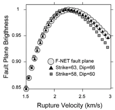
Using the methodology examined in the resolution test we calculated the total fault plane brightness for different rupture velocity values, as shown in Fig. 8. We can observe that the fault plane brightness has a clear peak for a rupture velocity value of 2.3 km/s, which would correspond to the optimumvalue for the Notohanto earthquake. To explore the stability of the solution, we tested different fault plane
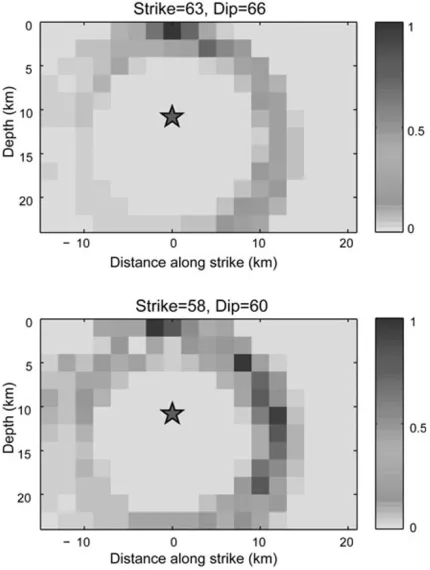
models by changing the fault strike to 63◦and the fault dip to 60◦, with respect to the F-NET solution. In all cases the optimum rupture velocity value is close to 2.3 km/s (Fig. 8). In the case of the asperity distribution result we found thatmodifying the strike by 5◦(with respect to the F-NET solution) did not significantly affect the source image solution, whereas a change by 6◦ in dip (with respect to the F-NET solution) introduced a defocusing effect into the source image (Fig. 9). This wouldmean that the fault plane corresponding to the F-NET solution leads to a better,more focused source image compared with the solutions for other fault plane geometries. For all themodels tested we found in general that the rupture velocity value estimated by IBM is very stable.
6.4 Source image computation time
One of themain advantages of the IBM source imaging is its very fast computation time. The calculation of a source
Fig. 6. EW component of velocity envelopes at K-NET and KiK-net sites used for source imaging, calculated frombandpass-filtered waveforms (1 to 30 Hz). The envelopes are aligned at the P-wave onset and ordered by increasing arrivals. The thick gray line represent the isochrone time corresponding to the largest asperity, by including a+/−1 s window around the isochrone.
Fig. 7. Horizontal projection of the fault plane brightness (color scale), overlapped by the first 24 h of aftershocks withmagnitude larger than 2 (black crosses). A yellow star depicts the JMA epicenter of the
mainshock and a black rectangle the fault planemodel used for source imaging.
using a conventional inversion procedure requires several hours of CPU time (Aoi and Sekiguchi, 2007). The total CPU time required for the IBM source imaging may be further reduced by calculating in advance tables of travel times for variable distances and source depths, at every K-NET and KiK-net station. This wouldmake IBM ideal for
Fig. 8. Normalized total fault plane brightness vs fault rupture veloc-ity. Source imaging solutions for three different fault plane geom e-tries are compared: circles correspond to the F-NET fault plane solution (Mw6.7, strike of 58◦and a dip of 66◦), triangles correspond to a fault
plane with a strike of 63◦and a dip of 66◦, and squares to a strike of 58◦ and a dip of 60◦.
quasi-real time estimation of an initial source process of earthquakes.
7.
Conclu
s
ion
s
Fig. 9. Fault plane brightness solution for a fault plane with a strike of 63◦ and a dip of 66◦(upper), and a fault plane with a strike of 58◦and a dip of 60◦(lower).
-Our source image of the Notohanto earthquake shows two large brigthness regions; the first region is located 10 kmabove the hypocenter along the dip and the second region is located near the bottomof the fault, NE of the hypocenter. These large brightness regions approximately correspond to large slip areas obtained by a standard source inversion approach. Our results demonstrate that IBM has the capability to quicklymap asperities of large earthquakes using observed strongmotion data and, therefore, could be suitable for a near-real time estimation of the source process of earthquakes.
-The rupture area of the Notohanto earthquake extended bilaterally 12 kmtowards the NE, and 6 kmtowards the SW along the strike. This fault area approximately corresponds with the largest concentration of aftershocks.
-We obtained an optimumfault rupture velocity value for the Notohanto earthquake of 2.3 km/s. Our results show that the IBM is able to provide stable estimates of fault rupture velocity.
-A sensibility analysis on the influence of fault geometry on the source imaging result shows that the fault plane cor-responding to the F-NET solution provides a well focused source image, compared with the results fromother fault plane geometries.
-The results of a resolution test show that the IBM is able to identify the location of large slip areas of earthquakes.
References
Allmann, B. and P. M. Shearer, A High-Frequency Secondary Event Dur-ing the 2004 Parkfield Earthquake,Science,318, 1279–1283, 2007. Aoi, S. and H. Sekiguchi, Rupture process of the 2005/3/25
Noto-Hanto Earthquake by using Near-fault dat a (preliminary version), http://www.kyoshin.bosai.go.jp/k-net/topics/noto070325/, 2007. Bernard, P. and R. Madariaga, A New Asymptotic Method for the
Model-ing of Near-Field Accelerograms,Bull. Seismol. Soc. Am.,74, 539–557, 1984.
Ellsworth, W. L., Imaging Fault Rupture Without Inversion,Seismol. Res Lett.,63, 73, 1992.
Festa, G., Slip imaging by isochron back projection and source dynamics with spectral elementmethods, Doctor thesis, University of Bologna and National Institute of Geophysics and Volcanology, pp. 195, 2004. Festa, G. and A. Zollo. Fault slip and rupture velocity inversion by
isochrone backprojection,Geophys. J. Int.,166, 745–756, 2006. Fletcher, J. B., P. Spudich, and L. M. Baker, Rupture Propagation of the
2004 Parkfield, California, Earthquake fromObservations at the UP-SAR,Bull. Seismol. Soc. Am.,96, S129–S142, 2006.
Hamada, M., O. Aydan, and A. Sakamoto, A quick report on Noto Peninsula earthquake on March 25, 2007, http://www.jsce-int.org/Report/Noto earthquake/Noto report.pdf, Japan Society of Civil Engineers, 2007.
Hartzell, S. and T. H. Heaton, Inversion of Strong Ground Motion and Teleseimic WaveformData for the Fault Rupture History of the 1979 Imperial Valley, California Earthquake, Bull. Seismol. Soc. Am.,73, 1553–1583, 1983.
Ishii, M., P. Shearer, H. Houston, and J. E. Vidale, Extent, duration and speed of the 2004 Sumatra-Andaman earthquake imaged by the Hi-Net array,Nature,435, 933–936, 2005.
Ito, K. and H. Wada, Observation ofmicroearthquakes in the Atotsugawa fault region, central Honshu, Japan seismicity in the creeping section of the fault, inSeismogenic Process Monitoring, edited by H. Ogasawara, T. Yanagidani, and M. Ando, 229–243, A. A. Balkema Publishers, Rot-terdam, 2002.
Iwata, T. and K. Irikura, Tomographic Imaging of Heterogeneous Rupture Process of a Fault Plane,Jisin,42, 49–58, 1989.
Kao, H. and S. J. Shan, Rapid identification of earthquake rupture plane using Source-Scanning Algorithm,Geophys. J. Int.,168, 1011–1020, 2007.
Sekiguchi, H., K. Irikura, and T. Iwata, Source inversion for estimating the continuous slip distribution on a fault—introduction of Green’s func-tions convolved with a correction function to givemoving dislocation effects in subfaults,Geophys. J. Int.,150, 377–391, 2002.
Spudich, P. and L. N. Frazer, Use of Ray Theory to Calculate High-frequency Radiation fromEarthquake Sources having Spatially Variable Rupture Velocity and Stress Drop,Bull. Seismol. Soc. Am.,74, 2061– 2082, 1984.
Spudich, P. and E. Cranswick, Direct observation of rupture propagation during the Imperial Valley earthquake using a short baseline accelerom -eter array,Bull. Seismol. Soc. Am.,74, 2083–2114, 1984.