R E S E A R C H
Open Access
On the Cauchy problem for a linear
harmonic oscillator with pure delay
Denys Ya Khusainov
1, Michael Pokojovy
2*and Elvin I Azizbayov
3*Correspondence:
[email protected] 2Department of Mathematics and Statistics, University of Konstanz, Konstanz, Germany
Full list of author information is available at the end of the article
Abstract
In the present paper, we consider a Cauchy problem for a linear second order in time abstract differential equation with pure delay. In the absence of delay, this problem, known as the harmonic oscillator, has a two-dimensional eigenspace so that the solution of the homogeneous problem can be written as a linear combination of these two eigenfunctions. As opposed to that, in the presence even of a small delay, the spectrum is infinite and a finite sum representation is not possible. Using a special function referred to as the delay exponential function, we give an explicit solution representation for the Cauchy problem associated with the linear oscillator with pure delay. Finally, the solution asymptotics as the delay parameter goes to zero is studied. In contrast to earlier works, no positivity conditions are imposed.
MSC: Primary 34K06; 39A06; 39B42; secondary 34K26
Keywords: functional-differential equations; harmonic oscillator; pure delay; well-posedness; solution representation
1 Introduction
LetXbe a (real or complex) Banach space and letx(t)∈Xdescribe the state of a physical system at timet≥. Witha(t) =x¨(t) denoting the acceleration of system, Newton’s second law of motion states that
F(t) =Ma(t) fort≥, ()
whereM: D(M)⊂X→Xis a linear, continuously invertible, accretive operator repre-senting the ‘mass’ of the system. When being displaced from its equilibrium situated in the origin, the system is affected by a restoring forceF(t). In classical mechanics, this force is postulated to be proportional to the instantaneous displacement,i.e.,
F(t) =Kx(t) fort≥ ()
for some closed, linear operatorK:D(K)⊂X→X. WhenM–Kis a bounded linear
op-erator, plugging Equation () into (), we arrive at the classical harmonic oscillator model
¨
x(t) =M–Kx(t) fort≥. ()
Assuming now that the restoring force is proportional to the value of the system at some past timet–τ, Equation () is replaced with the relation
F(t) =Kx(t–τ) fort≥, ()
whereτ > is a time delay. Plugging Equation () into () leads then to the linear harmonic oscillator equation with pure delay written as
¨
x(t) =M–Kx(t–τ) fort≥. ()
Problems similar to Equation () also arise when modeling systems with distributed pa-rameters such as general wave phenomena (cf.[]).
Equations similar to () are often referred to as delay or retarded differential equations. After being transformed to a first order in time system on a Banach space X, a general equation with constant delay can be written as
˙
u(t) =Ht,u(t),ut
fort> , u() =u, u=ϕ. ()
Here,τ> is a fixed delay parameter,ut:=u(t+·)∈L(–τ, ;X),t≥, denotes the his-tory variable,His anX-valued operator defined on a subset of [,∞)×X×L(–τ, ;X)
andu∈X,ϕ∈L(–τ, ;X) are appropriate initial data. Equations of type () have been
intensively studied in the literature. We refer the reader to the monographs by Els’gol’ts and Norkin [] and Hale and Lunel [] for a detailed treatment of Equation () in finite-dimensional spacesX. In contrast to this, results on Equation () in infinite-dimensional spacesXare less numerous. A good overview can be found in the monograph of Bátkai and Piazzera [].
Khusainovet al.considered in [] Equation () inRnwith
Ht,u(t),ut
=Au(t) +Au(t–τ) +
u(t)⊗b
u(t)
+u(t)⊗b
u(t–τ) +u(t–τ)⊗b
u(t–τ)
for symmetric matricesA,A∈Rn×nand column vectorsb,b,b∈Rnand proposed a
rational Lyapunov function to study the asymptotic stability of solutions to this system. In their work [], Khusainovet al.studied a modal, or spectrum, control problem for a linear delay equation onRnreading as
˙
x(t) =Ax(t) +bu(t) fort> ()
with a feedback controlu(t) =mj=cTjx(t–jτ) for some delay timeτ> and parameter vectorscj∈Rn. For canonical systems, they developed a method to compute the unknown parameters such that the closed-loop system possesses the spectrum prescribed before-hand. Under appropriate ‘concordance’ conditions, they were able to carry over their con-siderations for a rather broad class of non-canonical systems.
In the infinite-dimensional situation, a rather general particular case of () with
H(t,v,ψ) =Av+F(ψ), whereAgenerates aC-semigroup (S(t))t≥onXandFis a
appropriate assumptions on F, they proved the integral equation corresponding to the weak formulation of the delay equation given by
u(t) =S(t)ϕ() +
t
S(t–s)F(us) ds fort>
to possess a unique solution inH
loc(,∞;X).
Di Blasioet al.addressed in [] a similar problem
˙
u(t) = (A+B)u(t) +Lu(t–r) +Lut fort> , u() =u, u=ϕ, ()
whereAgenerates a holomorphicC-semigroup on a Hilbert spaceH,Bis a perturbation
ofAandL,Lare appropriate linear operators. Ifuandϕpossess a certain regularity,
they proved the existence of a unique strong solution inHloc (,∞;X)∩Lloc(,∞;D(A)) by analyzing theC-semigroup inducing the semiflowt →(u(t),ut). These results were elab-orated on by Di Blasioet al.in [] leading to a generalization for the case of weighted and interpolation spaces and including a description of the associated infinitesimal generator. Finally, the generalLp-case forp∈(,∞) was investigated by Di Blasio in [].
Diblíket al.[] studied Equation () for the case thatAandBare ×-second order and first order commuting differential operators, respectively, in a bounded interval (,l) ofR andL≡,L≡. Additionally, they allowed for non-homogeneous Dirichlet boundary
conditions. For this parabolic system, they proved the existence of solution in a class of classically differentiable functions both with respect to time and space under appropriate regularity conditions.
Recently, in their work [], Khusainovet al.proposed an explicitL-solution theory for a non-homogeneous initial-boundary value problem for an isotropic heat equation with constant delay
ut(t,x) =∂i
aij(x)∂ju(t,x)
+bi(x)∂iu(t,x) +c(x)u(t,x)
+∂i
˜
aij(x)∂ju(t–τ,x)
+b˜i(x)∂iu(t–τ,x) +˜c(x)u(t–τ,x)
+f(t,x) for (t,x)∈(,∞)×,
u(t,x) =γ(t,x) for (t,x)∈(,∞)×∂,
u(,x) =u(x) forx∈,
u(t,x) =ϕ(t,x) for (t,x)∈(–τ, )×,
where⊂Rdis a regular bounded domain and the coefficient functions are appropriate. Conditions assuring for exponential stability were also given.
Over the past decade, hyperbolic partial differential equations have attracted a con-siderable amount of attention, too. In [], Nicaise and Pignotti studied a homogeneous isotropic wave equation with an internal feedback with and without delay reading as
∂ttu(t,x) –u(t,x) +a∂tu(t,x) +a∂tu(t–τ,x) = for (t,x)∈(,∞)×,
u(t,x) = for (t,x)∈(,∞)×,
∂u
under the usual initial conditions where,⊂∂are relatively open in∂with¯∩
¯
=∅andνdenotes the outer unit normal vector of a smooth bounded domain⊂Rd.
They showed the problem to possess a unique global classical solution and proved the latter to be exponentially stable if a>a> or instable, otherwise. These results have
been carried over by Nicaise and Pignotti [] and Nicaiseet al.[] to the case of time-varying internally distributed or boundary delays.
In [], Khusainovet al.considered a non-homogeneous initial-boundary value problem for a one-dimensional wave equation with constant coefficients and a single constant delay
∂ttu(t,x) =a∂xxu(t–τ,x) +b∂xu(t–τ,x) +cu(t–τ,x)
+f(t,x) for (t,x)∈(,T)×(,l),
u(t,x) =γ(t,x) for (t,x)∈(,T)× {, },
u(,x) =u(x) forx∈(, ),
u(t,x) =ϕ(t,x) fort∈(–τ, ),x∈(, ).
Under appropriate regularity and compatibility assumptions, they proved the problem to possess a uniqueC-solution for any finiteT> . Their proof was based on extrapolation
methods forC-semigroups and an explicit solution representation formula.
Recently, Khusainov and Pokojovy presented in [] a Hilbert-space treatment of the initial-boundary value problem for the equations of thermoelasticity with pure delay
∂ttu(x,t) –a∂xxu(x,t–τ) +b∂xθ(x,t–τ) =f(x,t) forx∈,t> ,
∂tθ(x,t) –c∂xxθ(x,t–τ) +d∂txu(x,t–τ) =g(x,t) forx∈,t> ,
u(,t) =u(l,t) = , ∂xθ(,t) =∂xθ(l,t) = fort> ,
u(x, ) =u(x), u(x,t) =u(x,t) forx∈,t∈(–τ, ),
∂tu(x, ) =u(x), ∂tu(x,t) =u(x,t) forx∈,t∈(–τ, ),
θ(x, ) =θ(x), θ(x,t) =θ(x,t) forx∈,t∈(–τ, ).
Their proof exploited extrapolation techniques for strongly continuous semigroups and an explicit solution representation formula.
In the present paper, we give a Banach space solution theory for Equation () subject to appropriate initial conditions. Our approach is solely based on the step method and does not incorporate any semigroup techniques. In contrast to earlier works by Khusainovet al.
[, , ], we only require the invertibility and not the negativity ofM–Kin Equation ().
In this sense, our framework is different from that employed by Diblíket al.in [, ], as they required the coefficient matrices to be negative definite. It should though be pointed out that their solution theory accounted for two and more delays, whereas we consider a single delay.
the delayed exponential function introduced by Khusainov and Shuklin in []. Finally, we prove the solution of the delay equation to converge to the solution of the original second order abstract differential equation as the delay parameterτ goes to zero.
2 Classical harmonic oscillator
For the sake of completeness, we briefly discuss the initial value problem for the harmonic oscillator being a second order in time abstract differential equation
¨
x(t) –x(t) =f(t) fort≥ ()
subject to the initial conditions
x() =x∈D(), x˙() =x∈X. ()
Here, we assume the linear operator:D()⊂X→Xto be continuously invertible and generate aC-group (et)t∈R⊂L(X) on a (real or complex) Banach spaceXwith L(X)
denoting the space of bounded, linear operators onXequipped with the normAL(X):=
sup{AxX:x∈X,xX≤}. A more rigorous treatment of this problem can be found in [], Section ..
The general solution to the homogeneous equation is known to read as
xh(t) =etc+e–tc fort≥
with somec,c∈D(). Vectorsc,ccan be computed using the initial conditions from
Equation () leading to a system of linear operator equations
c+c=x, c–c=x.
The latter is uniquely solved by
c=
–(x
+x), c=
–(x –x).
Thus, the unique solution of the homogeneous equation with the initial conditions () is given by
xh(t) =
–et(x
+x) +
–e–t(x
–x) fort≥ ()
or, equivalently,
xh(t) =
et+e–tx+
–et–e–tx
fort≥. ()
A particular solution to the non-homogeneous equation with zero initial conditions will be determined in the Cauchy form
xp(t) =
t
K(t,s)f(s) ds fort≥. ()
ker-nel,i.e., for any fixeds≥, the functionK(·,s) is the solution of the homogeneous problem
Solving this system with generalized Cramer’s rule, we obtain, fors≥,
c(s) =
Thus, the Cauchy kernel is given by
K(t,s) =
–e(t–s)–e–(t–s) fort,s≥,
whereas the particular solution satisfying zero initial conditions reads as
xp(t) = D()), then the mild solutionxgiven in Equation () is a classical solution satisfying
x∈C([,∞),X)∩C([,∞),D())∩C([,∞),D()).
3 The linear oscillator with pure delay
In this section, we consider a Cauchy problem for the linear oscillator with a single pure delay
¨
subject to the initial condition
x(t) =ϕ(t) fort∈[–τ, ]. ()
Here,Xis a Banach space,∈L(X) is a bounded, linear operator andϕ∈C([–τ, ],X), f ∈L
loc(,∞;X) are given functions. In contrast to the previous section, the boundedness
ofis indispensable here. Indeed, Dreheret al.proved in [] that Equations ()-() are ill-posed even ifXis a Hilbert space andpossesses a sequence of eigenvalues (λn)n∈N⊂
Rwithλn→ ∞orλn→–∞asn→ ∞. The necessity forbeing bounded has also been pointed out by Rodrigueset al.in [] when treating a linear heat equation with pure delay.
Definition A functionx∈C([–τ,∞),X)∩C([–τ, ],X)∩C([,∞),X) satisfying
Equations ()-() pointwise is called a classical solution to the Cauchy problem ()-().
A mild formulation of ()-() is given by
˙
x(t) =x˙() +
t
x(s– τ) ds+
t
f(s) ds fort≥, ()
x(t) =ϕ(t) fort∈[–τ, ]. ()
Definition A functionx∈C([–τ,∞),X) satisfying Equations ()-() is called a mild
solution to the Cauchy problem ()-().
By the virtue of fundamental theorem of calculus, any mild solutionxto ()-() with
x∈C([–τ,∞),X)∩C([–τ, ],X)∩C([,∞),X) is also a classical solution.
Obvi-ously, for the problem ()-() to possess a classical solution, one necessarily requires ϕ∈C([–τ, ],X).
In the following subsection, we want to study the existence and uniqueness of mild and classical solutions to the Cauchy problem ()-() as well as their continuous dependence on the data.
3.1 Existence and uniqueness
Rather than using the semigroup approach (cf.[], Chapter ), we decided to use the more straightforward step method here reducing ()-() to a difference equation on the func-tional vector spaceCˆ
τ(N,X) defined as follows.
Definition LetXbe a Banach space,τ> ands∈N. We introduce the metric vector
space
ˆ
Cτs(N,X) :=l∞loc
N,Cs
[–τ, ],X
:=
x= (xn)n∈N xn∈C
s[–τ, ],Xforn∈N
,
dj
dtjxn(–τ) = dj
dtjxn–() forj= , . . . ,s– ,n∈N
equipped with the distance function
dCˆτs(N,X)(x,y) :=
n∈N
–n maxk=,...,nxk–ykCs([–τ,],X)
+maxk=,...,nxk–ykCs([–τ,],X) forx,y∈ ˆC
s τ(N,X).
Obviously,Cˆτs(N,X) is a complete metric space which is isometrically isomorphic to
the metric spaceCs
τ([–τ,∞),X) :=Cs([–τ,∞),X) equipped with the distance
dCτs([,∞),X)(x,y) :=
n∈N
–n x–yCs([–τ,τn],X)
+x–yCs([–τ,τn],X) forx,y∈C
s[–τ,∞),X.
For anyx: [–τ,∞)→X, we define forn∈Nthenth segment ofxvia
xn:=x(nτ+s) fors∈[–τ, ].
By induction,xis a mild solution of ()-() if and only if (xn)n∈N∈ ˆC
τ(N,X) solves
˙
xn(s) =x˙n–() +
s
–τ
xn–(σ) dσ
+
nτ+s
(n–)τ
f(σ) dσ fors∈[–τ, ] andn∈N, ()
x(s) =ϕ(s) fors∈[–τ, ].
Theorem Equation()has a unique solution(xn)n∈N∈ ˆCτ(N,X).Moreover,x con-tinuously depends on the data in sense of the estimate
xnC([–τ,],X)≤κn
ϕC([–τ,],X)+fL(,τn;X)
for any n∈N
withκ:= + τ( + τ)( +
L(X)).
Proof By the virtue of fundamental theorem of calculus, Equation () is satisfied if and only if
xn(s) =xn–() + (s+ τ)x˙n–() +
s
–τ
σ
–τ
xn–(ξ) dξdσ
+
s
–τ
nτ+σ
(n–)τ
f(ξ) dξdσ fors∈[–τ, ],n∈N, ()
xn(–τ) =xn–(), x˙n(–τ) =x˙n–() forn∈N, ()
x(s) =ϕ(s) fors∈[–τ, ]. ()
By induction, we can easily show that for any n∈Nthere exists a unique local solu-tion (x,x, . . . ,xn)∈(C([–τ, ],X))n+to ()-() up to the indexn. Here, we used the
Sobolev embedding theorem stating
Further, we can estimate
Equations () and () imply together
xnC([–τ,],X)≤κ
which finishes the proof.
Lettingx(t) :=xk(t– kτ) fort≥ andk:=tτ ∈N, we obtain the unique mild
solu-tionxof Equations ()-().
Corollary Equations()-()possess a unique mild solution x satisfying,for any T:= nτ,n∈N,
Proof Differentiating Equation () with respect tot, using the assumptions and the fact thatx∈C([–τ,∞),X), we deduce thatx|[–τ,]≡ϕ∈C([–τ, ],X) and
¨
x=x(·– τ) +f∈C[,∞),X.
Hence,x∈C([–τ,∞),X)∩C([–τ, ],X)∩C([,∞),X) and is thus a classical solution
of Equations ()-().
3.2 Explicit representation of solutions
Throughout this section, we additionally assume that: X→X is an isomorphism from the Banach spaceXonto itself.
Theorem The delayed exponential functionexpτ(·;)lies in C([–τ,∞),X)∩C([,
Proof To prove the smoothness ofx, we first note thatxis an operator-valued polyno-mial and thus analytic on each of the intervals [(k– )τ,kτ] fork∈Z. By the definition of
Fort≥τ, differentiation yields
Corollary The delayed exponential functionexpτ(·; –)lies in C([–τ,∞),X)∩C([,
As we already pointed out in the introduction section, in contrast to earlier works by Khusainovet al.[, , ], only the invertibility and not the negativity ofis necessary for our purposes.
From Equation (), we explicitly obtain
xτ(t;) =
Theorem The functions x
τ(·;), xτ(·;) have the following regularity properties:
x
τ(·;),xτ(·;)∈C([–τ,∞),X)∩C([–τ, ],X)∩C([τ,∞),X). Further, xτ(·;) and
xτ(·;) are solutions to the Cauchy problem ()-()with the initial dataϕ(t) = idX, –τ≤t≤τ,andϕ(t) = L(X), –τ≤t≤τ,respectively.
First, assumingf ≡X, Equations ()-() reduce to
¨
x(t) –x(t– τ) = fort≥, ()
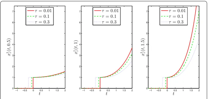
Figure 1 Plot ofx1
τ(·;) function.
Figure 2 Plot ofx2
τ(·;) function.
Theorem Letϕ∈C([–τ, ],X).Then the unique classical solution x to the Cauchy
problem()-()is given by
x(t) =xτ(t+τ;)ϕ(–τ) +xτ(t+ τ;)ϕ˙(–τ)
+
–τ
xτ(t–s;)ϕ¨(s) ds.
Proof To solve Equations ()-(), we use the ansatz
x(t) =xτ(t+τ;)c+xτ(t+ τ;)c
+
–τ
xτ(t–s;)¨c(s) ds ()
Plugging the ansatz from Equation () into Equation (), we obtain, fort≥,
and¨cvanish implying that the functionxin Equation () is a solution of Equation (). Now, we show that selectingc:=ϕ(–τ),c:=ϕ˙(–τ) andc:=ϕ, the functionxin
Equa-Exploiting the fact thatx
τ vanishes on [–τ, ], we get
[Iϕ](t) =
t+τ
xτ(σ;)ϕ¨(t–σ) dσ.
Integrating by parts, we further get
we obtain
[Iϕ](t) = –xτ(t+ τ;)ϕ˙(–τ) +
t+τ
˙
xτ(σ;)ϕ˙(t–σ) dσ.
Again, using Equation () and
xτ(t;) = idX, –τ≤t≤τ,
we compute
[Iϕ](t) = –xτ(t+ τ;)ϕ˙(–τ) +
t+τ
˙
ϕ(t–σ) dσ
= –xτ(t+ τ;)ϕ˙(–τ) –ϕ(t–σ)| σ=t+τ σ=
= –xτ(t+ τ;)ϕ˙(–τ) –xτ(t+τ;)ϕ(–τ) +ϕ(t).
Hence, fort∈[–τ, ], we have
x(t) =xτ(t+τ;)ϕ(–τ) +xτ(t+ τ;)ϕ˙(–τ) +
–τ
xτ(t–s;)ϕ¨(s) ds=ϕ(t)
as claimed.
Next, we consider Equations ()-() for the trivial initial data,i.e.,
¨
x(t) –x(t– τ) =f(t) fort≥, ()
x(t) = fort∈[–τ, ]. ()
Theorem Let f ∈C([,∞),X).The unique classical solution x to the Cauchy problem
()-()is given by
x(t) =
t
xτ(t–s;)f(s) ds.
Proof To find an explicit solution representation, we use the ansatz
x(t) =
t
xτ(t–s;)c(s) ds fort≥τ
for some functionc∈C([,∞),X). Differentiating this expression with respect totand
exploiting the initial conditions forx
τ(·;), we get
˙
x(t) =
t
˙
xτ(t–s;)c(s) ds+xτ(t–s;)c(s)|s=t
=
t
˙
xτ(t–s;)c(s) ds+xτ()c(t)
=
t
˙
Differentiating again, we find
¨
x(t) =
t
¨
xτ(t–s;)c(s) ds+x˙τ(t–s;)c(s)|s=t
=
t
¨
xτ(t–s;)c(s) ds+x˙τ(+;)c(t)
=
t
¨
xτ(t–s;)c(s) ds+c(t).
Plugging this into Equation () and recalling thatxτ(·;) is a solution of the homogeneous equation, we get
c(t) +
t
¨
xτ(t–s;) –xτ(t– τ–s;)
c(s) ds=f(t)
and thereforec≡f.
As a consequence from Theorems and , we obtain using the linearity property of Equations ()-() the following.
Theorem Letϕ∈C([–τ, ],X)and f ∈C([,∞),X).The unique classical solution
to Equations()-()is given by
x(t) =xτ(t+τ;)ϕ(–τ) +xτ(t+ τ;)ϕ˙(–τ) +
–τ
xτ(t–s;)ϕ¨(s) ds
+
, t∈[–τ, ),
t
x
τ(t–s;)f(s) ds, t≥
for t∈[–τ,∞).
Finally, after a partial integration, we get the following.
Theorem Letϕ∈C([–τ, ],X)and f ∈L
loc(,∞;X).The unique mild solution to Equations()-()is given by
x(t) =xτ(t+τ;)ϕ(–τ) +xτ(t;)ϕ˙() –
–τ
˙
xτ(t–s;)ϕ˙(s) ds
+
, t∈[–τ, ),
t
x
τ(t–s;)f(s) ds, t≥
for t∈[–τ,∞).
3.3 Asymptotic behavior as
τ
→0Again, we assumeXto be a Banach space and prove the following generalization of Lem-ma in [].
Proof First, we want to exploit the mathematical induction to show, for anyk∈N,
expτ(t–τ;) –exp(t)L(X)≤τL(X)exp
value theorem for Bochner integration since
+L(X)
Proof Lemma and the mean value theorem for Bochner integration yield
expτ(t+γ;) –etL(X)
Theorem Letτ> .For anyτ ∈(,τ),let x(·;τ)denote the unique mild solution of
Proof Using the explicit representation of the mild solutionx¯andx(·;τ), respectively, we can estimate
Hence, the claim follows.
Corollary Under conditions of Theorem,we additionally have
Proof Integrating Equation () and using Equation () as well as exploiting Equations ()-() yields
x˙(t;τ) –x˙¯(t)X≤ϕ˙(;τ) –xX+
t
x(s– τ;τ) –x¯(s)Xds
≤I,(t) +I,(t) +I,(t) fort∈[,T]
with
I,(t) :=ϕ˙(;τ) –xX, I,:=L(X)
–τ
ϕ(s) –x¯(s+ τ)Xds,
I,(t) :=L(X)
t
τ
x(s– τ;τ) –x¯(s)Xds.
Taking into account Equation (), we can estimate
¯xC([,τ],X)≤
x+–L(X)x
eL(X)T
+– L(X)e
L(X)TfL (,T;X).
Hence,
I,(t)≤δτ
ϕC([,T],X)+xX+xX+fL(,T;X)
.
Applying Theorem , we further get
I,(t)≤L(X)Tβϕ(–τ;τ) –xX+ϕ˙(;τ) –xX
+τϕ(·;τ)C([–τ,],X)+fL(,T;X)
.
Combining these inequalities and using again Theorem , we deduce the estimate
as-serted.
Competing interests
The authors declare that they have no competing interests.
Authors’ contributions
All authors equally contributed to the problem discussion and writing the introduction section. DK proved the explicit solution representation formula for the harmonic oscillator with pure delay. MP showed the abstract well-posedness for the harmonic oscillator with pure delay and studied its asymptotics as the delay parameter goes to zero. EA presented a study on the classical harmonic oscillator without delay as well as checked the proofs and verified the calculations. All the authors read and approved the final manuscript.
Author details
1Faculty of Cybernetics, Kyiv National Taras Shevchenko University, Kyiv, Ukraine.2Department of Mathematics and Statistics, University of Konstanz, Konstanz, Germany.3Faculty of Mechanics and Mathematics, Baku State University, Baku, Azerbaijan.
Acknowledgements
The authors would like to express their deep gratitude to the editorial team and the anonymous referees for the careful reading of the manuscript as well as their valuable comments and suggestions which helped to improve the present paper. The kind financial support from the Young Scholar Fund at the University of Konstanz, Konstanz, Germany (Deutsche Forschungsgemeinschaft ZUK 52/2 grant) is greatly appreciated.
References
1. Khusainov, D, Pokojovy, M, Azizbayov, E: Representation of classical solutions to a linear wave equation with pure delay. Bull. Kyiv Natl. Univ., Ser. Cybern.13, 5-12 (2013)
2. Els’gol’ts, LE, Norkin, S: Introduction to the Theory and Application of Differential Equations with Deviating Arguments. Mathematics in Science and Engineering, vol. 105. Elsevier, Burlington (1973)
3. Hale, J, Lunel, S: Introduction to Functional Differential Equations. Springer, New York (1993)
4. Bátkai, A, Piazzera, S: Semigroups for Delay Equations. Research Notes in Mathematics, vol. 10. AK Peters, Wellesley (2005)
5. Khusainov, D, Agarwal, R, Davidov, V: Stability and estimates for the convergence of solutions for systems involving quadratic terms with constant deviating arguments. Comput. Math. Appl.38, 141-149 (1999)
6. Khusainov, D, Agarwal, R, Kosarevskaya, N, Kojametov, A: Spectrum control in linear stationary systems with delay. Comput. Math. Appl.39, 39-55 (2000)
7. Travies, C, Webb, G: Partial differential equations with deviating arguments in the time variable. J. Math. Anal. Appl.
56(2), 397-409 (1976)
8. Di Blasio, G, Kunisch, K, Sinestari, E: The solution operator for a partial differential equation with delay. Atti Accad. Naz. Lincei, Rend. Cl. Sci. Fis. Mat. Nat.74(4), 228-233 (1983)
9. Di Blasio, G, Kunisch, K, Sinestari, E:L2-Regularity for parabolic partial integro-differential equations with delay in the highest-order derivatives. J. Math. Anal. Appl.102(1), 38-57 (1984)
10. Di Blasio, G: Delay differential equations with unbounded operators acting on delay terms. Nonlinear Anal.52(1), 1-18 (2003)
11. Diblík, J, Khusainov, D, Kukharenko, O, Svoboda, Z: Solution of the first boundary-value problem for a system of autonomous second-order linear partial differential equations of parabolic type with a single delay. Abstr. Appl. Anal.
2012, Article ID 219040 (2012)
12. Khusainov, D, Pokojovy, M, Racke, R: Strong and mild extrapolatedL2-solutions to the heat equation with constant delay. SIAM J. Math. Anal.47(1), 427-454 (2015)
13. Nicaise, S, Pignotti, C: Stability and instability results of the wave equation with a delay term in the boundary or internal feedbacks. SIAM J. Control Optim.45(5), 1561-1585 (2006)
14. Nicaise, S, Pignotti, C: Stabilization of the wave equation with boundary or internal distributed delay. Differ. Integral Equ.21(9-10), 935-958 (2008)
15. Nicaise, S, Pignotti, C, Valein, J: Exponential stability of the wave equation with boundary time-varying delay. Discrete Contin. Dyn. Syst., Ser. S4, 693-722 (2011)
16. Khusainov, D, Pokojovy, M: Solving the linear 1D thermoelasticity equations with pure delay. Int. J. Math. Math. Sci.
2015, Article ID 479267 (2015)
17. Khusainov, D, Diblík, J, R˚u˘zi˘cková, M, Luká˘cová, J: Representation of a solution of the Cauchy problem for an oscillating system with pure delay. Nonlinear Oscil.11(2), 276-285 (2008)
18. Khusainov, D, Ivanov, A, Kovarzh, I: The solution of wave equation with delay. Bull. Taras Shevchenko Natl. Univ. Kyiv., Ser. Phys. Math.4, 243-248 (2006) (in Ukrainian)
19. Diblík, J, Feˇckan, M, Pospıšil, M: Representation of a solution of the Cauchy problem for an oscillating system with two delays and permutable matrices. Ukr. Math. J.65, 58-69 (2013)
20. Diblík, J, Feˇckan, M, Pospıšil, M: Representation of a solution of the Cauchy problem for an oscillating system with multiple delays and pairwise permutable matrices. Abstr. Appl. Anal.2013, Article ID 931493 (2013)
21. Khusainov, D, Shuklin, G: On relative controllability in systems with pure delay. Prikl. Mekh.41(2), 118-130 (2005) 22. Arendt, W, Batty, C, Hieber, M, Neubrander, F: Vector-Valued Laplace Transforms and Cauchy Problems. Monographs
in Mathematics, vol. 96. Birkhäuser, Basel (2001)
23. Dreher, M, Quintanilla, R, Racke, R: Ill-posed problems in thermomechanics. Appl. Math. Lett.22(9), 1374-1379 (2009) 24. Rodrigues, H, Ou, C, Wu, J: A partial differential equation with delayed diffusion. Dyn. Contin. Discrete Impuls. Syst.,