R E S E A R C H
Open Access
A cognitive QoS management framework for
WLANs
Mostafa Pakparvar
*, David Plets, Emmeric Tanghe, Dirk Deschrijver, Wei Liu, Krishnan Chemmangat,
Ingrid Moerman, Tom Dhaene, Luc Martens and Wout Joseph
Abstract
Due to the precipitous growth of wireless networks and the paucity of spectrum, more interference is imposed to the wireless terminals which constraints their performance. In order to preserve such performance degradation, this paper proposes a framework which uses cognitive radio techniques for quality of service (QoS) management of wireless local area networks (LANs). The framework incorporates radio environment maps as input to a cognitive decision engine that steers the network to optimize its QoS parameters such as throughput. A novel experimentally verified heuristic physical model is developed to predict and optimize the throughput of wireless terminals. The framework was applied to realistic stationary and time-variant interference scenarios where an average throughput gain of 344% was achieved in the stationary interference scenario and 70% to 183% was gained in the time-variant interference scenario.
Keywords: Dynamic spectrum access; Radio environment maps; Cognitive radios; Interference management
1 Introduction
Large-scale growth of wireless networks and spectrum scarcity are introducing more interference than ever. Intensive interference degrades wireless links and may jeopardize continuous connectivity and hence quality of service (QoS) offered to the users.
Cognitive radios (CRs) are becoming a tempting solu-tion to tackle this type of spectrum over-utilizasolu-tion by introducing opportunistic usage of frequency bands that are not heavily occupied by licensed users [1]. The equal regulatory status of wireless terminals on the industrial scientific medical (ISM) band leaves no consideration of a primary user for various wireless networks. Therefore, interoperability of ISM band networks is becoming a key issue that must be solved.
Wireless networks are designed to tackle homogeneous intra/inter network interference by means of various medium access techniques. The efficiency of interference-tackling techniques of the present wireless technolo-gies has been profoundly assessed in the literature. For instance in [2], a large number of experiments prove that the throughput of IEEE 802.11 wireless local area network
*Correspondence: mostafa.pakparvar@intec.ugent.be
Department of Information Technology (INTEC), Ghent University-iMinds, Gaston Crommenlaan 8 box 201, Gent 9050, Belgium
(WLAN) is highly dependent on the traffic characteristics of other present Wi-Fi networks.
The objective of this paper is to validate a framework that uses cognitive radio techniques for QoS manage-ment of WLANs. Cognitive radio techniques are majorly studied and practiced for operation of secondary users in licensed bands while this framework focuses on deploy-ing such techniques in the unlicensed ISM band. The framework builds on radio environment maps (REMs) that contain PHY spectrum information obtained from a set of environment sensing devices. An experimentally verified heuristic physical model is developed to predict and optimize the throughput of wireless terminals based on the information contained in the REMs. The model is used as the kernel of the cognitive decision engine (CDE). The novelties presented in this paper are the following: (1) extendable real-time indoor radio environment maps: maps that can be redesigned for any indoor environment, and (2) an experimentally verified heuristic cognitive deci-sion engine which is based on a physical model that predicts throughput as a function of measurable wireless LAN parameters.
The model is derived from a set of exploratory ments and is validated with various practical measure-ments in a pseudo shielded experimental testbed building, w-iLab.t [3].
The rest of this paper is organized as follows. In Section 2, after reviewing the related works, the cog-nitive framework is outlined. Section 3 describes a set of exploratory measurements we performed to derive a heuristic physical model which servers as the kernel of the cognitive decision engine. In Section 4, the development of the heuristic model is elaborated, and in Section 5, we explain how this model is integrated to the cognitive deci-sion engine. Section 6 presents two proof of concept sce-narios for static and time variant interference. Section 7 demonstrates an application outlook of the framework. Section 8 presents the conclusions.
2 The cognitive framework 2.1 Related work
In the context of cognitive frameworks that address effi-cient interoperability of homo/heterogeneous wireless networks, spectrum monitoring and decision making are the central topics addressed by the authors in the cur-rent literature. REMs [4] play a key role for environment monitoring in many cognitive radio solutions. REMs rep-resent an integrated database providing information such as spectrum availability, regulations, and also the degree of channel utilization [4]. In terms of spectrum utilization, REMs have been proposed to measure power spectral density (PSD) in order to determine the degree of spec-trum utilization in a certain geographical area. These models are produced from a set of measurements and the application of spatial interpolation techniques that provide an estimate at locations that lack dedicated mea-surements [5]. In addition to PSD maps, other authors present channel gain maps that capture information about the propagation medium [6]. In [7], the authors propose using medium utilization as a metric to be included in the REMs dedicated for wireless LANs. In [8], REMs have been used to intelligently guide spectrum access for deployment of a prototype of a long-term evolution (LTE) system that opportunistically exploits the spectral white spaces in the upper ultra high frequency (UHF) TV bands. The decision making mechanisms in the present lit-erature exploit a multitude of artificial intelligence (AI) algorithms to derive proper decisions for operation of the cognitive wireless network. artificial neural networks (ANN) have been used for radio parameter adaptation in CR [9,10]. The ANN determines radio parameters for given channel states with three optimization goals, includ-ing meetinclud-ing the bit error rate (BER), maximizinclud-ing the throughput, and minimizing the transmit power. In [11], it is proposed that the use of ANN characterizes the real-time achievable communication performance in CR. Since the characterization is based on runtime measure-ments, it provides a certain learning capability that can be exploited by the cognitive engine. The simulation results
demonstrate good modeling accuracy and flexibility in various applications and scenarios.
Metaheuristics [12] are used for combinatorial opti-mization in which an optimal solution is sought over a discrete search space. Evolutionary algorithms/genetic algorithms (GAs), simulated annealing (SA), tabu search (TS), and ant colony optimization (ACO) are examples of metaheuristic algorithms. Among the various meta-heuristic algorithms, the GA has been widely adopted to solve multiobjective optimization problems and to dynamically configure the CR in response to the chang-ing wireless environment [13,14]. For instance in [14], a software testbed for CR with the spectrum-sensing capa-bility is implemented and a GA-based cognitive engine to optimize radio parameters for dynamic spectrum access is validated.
Apart from all the aforementioned AI methods, there are also methods in the literature that are based upon ranking the channels in order of their capacity. The ranking is done by characterizing the channel activities and making estimations of the capacity accordingly. For instance, in [15], the authors derive aphysical modelfor the throughput of WiMax networks based on monitor-ing physical layer parameter carrier to interference and noise ratio (CINR). In particular, the authors in [16] pro-pose a spectrum decision framework for cognitive radio networks which addresses QoS management of the sec-ondary users in response to certain events such as appear-ance of a primary user or degradation of the QoS. Thus, their proposed framework not only accounts for consider-ation of primary users but also maintains the QoS deliv-ered to the secondary users by making spectrum decision according to the channel activities. The current paper is therefore a logical continuance and extension of [16] where we share a common architecture for tackling inter-ference and optimizing the QoS. We extend the concept by bringing cognitive radio techniques for QoS manage-ment to the ISM band WLANs as well as incorporating radio environment maps to the framework. To this end, we have extended the framework by adding radio environ-ment maps and a cognitive decision engine which utilizes a physical throughput model to estimate and optimize the throughput of the IEEE 802.11 network.
2.2 Setup architecture
The architecture of the cognitive framework is illustrated in Figure 1.
DB
REM Decision
Engine
Network controller
Elements of network under study
Interference sources
Figure 1Architecture of the framework.
be monitored and processed in order to make proper decisions to optimize the QoS.
2.3 Construction of the radio environment map
REMs [4] in this framework (Figure 1) refer to real-time spatial maps of the spectrum. These maps display vital information on spectral utilization across the whole net-work. As such, they facilitate environment monitoring by presenting relevant parameters that will be elaborated in Section 2.5. REMs can also be used by authorities to mon-itor spectrum for either finding violations of regulations or finding the so-called white spaces of the spectrum. For instance, apart from the real-life implementation of REMs in [6], the IEEE 802.22 standard [17] recommends the authorities to prepare database services (similar to REMs) to provide public access to query for available TV channels. Indoor REMs give unprecedented insight on spectrum utilization in buildings with highly dense exploitation of wireless terminals.
Monitoring of spectrum in the wireless environment is a crucial part of any cognitive radio solution.
There are various solutions that enable wireless envi-ronment monitoring. Software-defined radios (SDRs) are advanced devices that are highly utilized within the cog-nitive radio networks for monitoring the intended bands [18]. Packet sniffers are an alternative solution used for monitoring the activity of a certain wireless technology on a certain band. Combining several packet sniffers on the different intended channels will bring the same func-tionality of a single software-defined radio device. The low cost and simplicity of implementation in case of the Fi technology is our motivation to only consider Wi-Fi packet sniffers as sources providing information of the spectrum.
The availability of information sources is restricted to a sparse set of (discrete) locations in the environment
which necessitates utilizing interpolation techniques to estimate data values at arbitrary locations of the map. To this end, the architecture of the REM is designed as illus-trated in Figure 2. The interpolation engine will extract raw data from the database in order to build an interpola-tion model. To preserve generality, the design foresees the feature for the user to select the appropriate interpolation technique according to their hardware and other require-ments. The other input argument of the interpolation engine is the resolution of the interpolation that defines the number of points that must be interpolated based on the limited measured points. The interpolation method that is used in this paper by the REM is inverse distance weighting (IDW) [19]. This choice is motivated by the simplicity of underlying principle and the speed in calcu-lation. The REM is implemented in the WiCa Heuristic Indoor Propagation Prediction tool [20].
2.4 The cognitive decision engine
The CDE in this framework (see Figure 1) refers to the entity that reconfigures the network with informed deci-sions that are based on its observation and cognition of the REMs. The architecture of the CDE is illustrated in Figure 3. The decision maker, in general, could be replaced by a human network manager or an automatic cognitive algorithm. The resource manager steers the network in response to the following events:
• Connection request: when a new connection is requested from the user.
• QoS degradation: when the clients of network under test report degraded quality of service.
• Sensing event: when the network under test is not active, this event keeps the decision maker informed of the channel quality on different bands.
The decision maker in this paper depends on a physical model that estimates the throughput based on interfer-ence observation. The decision maker invokes the models on the intended bands of operation and ranks the chan-nels according to the estimations. The development of the physical model is further explained in Section 4.
2.5 Parameters
The different parameters that affect the performance of the wireless system can be classified as follows:
• Uncontrollable parameters: time-varying parameters that can be measured or monitored in the network but cannot be modified directly by the decision engine. They are further subdivided into two classes:
Figure 2Interpolation architecture.
throughput, latency, jitter, packet loss, mean opinion score (MOS)).
– Measurable parameters (meters): these are the parameters that define the wireless environment and ‘state’ of the wireless system. These parameters are mostly informative (e.g., received signal strength indicator (RSSI) values, channel occupancy).
• Controllable parameters (knobs): configurable parameters that can be tuned or controlled by the cognitive decision engine (e.g., transmit power, packet size, location of the wireless entity).
The optimization process uses the knobs to optimize its target parameters given the input parameters (meters). This classification is shown in Table 1. Interference is the major issue that causes QoS degradation of wireless networks. Therefore, it should be characterized spatially, spectrally, and temporally in order to understand its influ-ence on the QoS parameters. Table 1 also represents parameters that characterize interference. Parameters fol-lowed by a superscripted letter ‘a’ are those that are used in this research for deriving a model that predicts the throughput of a wireless network given the present inter-ference characteristics.
Selection of the knobs in Table 1 is limited to the con-trollable parameters of IEEE 802.11g interfaces in the test environment which will be described in Section 3.1.1.
Quality Monitoring
Spectrum Sensing Resource Manager
Decision Maker
Network Controller
Event Detector
To the network
From REM Connection
request
Figure 3The architecture of the cognitive decision engine.
Packet size is not considered since it is set primarily by the application and consequently controlled by the IP layer in a process called IP fragmentation to make sure it does not exceed the maximum transmission unit (MTU) [21]. The 1470 UDP packet size is used to avoid fragmentation of the packets.
Considering the audiovisual application of the network, instead of a QoS parameter, one may target a quality of experience (QoE) metric like mean opinion score (MOS) for audio or video streams. The audio MOS depends on QoS parameters, namely latency, jitter, and packet loss [22]. Finally, all meters are useful parameters to be repre-sented on radio environment maps.
3 Exploratory measurements
After describing the network configuration and the exper-iment setup, we will explain the exploratory measure-ment campaigns we performed for deriving the physical model of the throughput. Each measurement campaign aims at studying the influence of measurable interference characteristics on the throughput of the network under study.
3.1 Experiment description
3.1.1 Network configuration
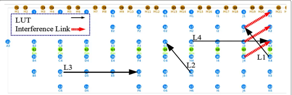
All experiments are conducted in a pseudo-shielded testbed environment [3] in Ghent, Belgium. The nodes in the testbed are mounted in an open room (66 m × 20.5 m) in a grid configuration with an x-separation of 6 m and a y-separation of 3.6 m. Figure 4 shows the ground plan of the test lab with an indication of the location of the nodes. The 60 installed nodes are represented by the blue locations on the picture. Each node has two Wi-Fi interfaces (Sparklan WPEA-110N/E/11n mini PCIe 2T2R chipset: AR9280). Further-more, a ZigBee sensor node and a USB 2.0 Bluetooth interface (Micro CI2v3.0 EDR) are incorporated into each node.
3.1.2 Experiment setup
Table 1 Optimization parameters
Knobs (controllable) Values Unit Meters (uncontrollable) Unit Target
Transmission Network under test QoS
Data generation rate [0-54] Mbps Latency ms Latency
Transmission rate [1,2,11,18,24,36,48,54] Mbps Jitter ms Jitter
Packet size 1,470 Bytes Throughput (T) Mbps Throughput
Frequency channel [1-13]a Packet loss % Packet loss
Power [0-20]a dBm Interference network QoE
Channel occupancy degreea % MOS
Location Interference TxRatea Mbps
(x,y) coordinate Meters Interference power levela dBm
Height Meters Interference channela
aThe parameters considered in the application of this paper.
second phase where interference is generated in the envi-ronment. Phase 2 of each experiment proceeds as fol-lows: a. Start the interference transmission, b. wait 1 s to ensure interference is on the air, c. start the link-under-test transmission for nseconds, d. wait n seconds, and e. stop all data transmissions. The value of n specified for each measurement is mentioned at the correspond-ing measurement description. Data generation for the interference link and the link under test has been facil-itated by the iperf traffic generator tool [23]. Using a client-server configuration, iperf outputs periodic reports of the throughput. Reports are parsed and stored in a database on the experiment controller server of the testbed.
During each interference measurement, two connection links are established, as displayed in Figure 4. The first link, always operating on channel 6, is denoted as the link under test (LUT). By default, this link is set at loca-tion L1 (see Figure 4) unless otherwise menloca-tioned. The second link is the interfering link, between node 30 and node 20 (see IL1 in Figure 4). The data generation rate of
the transmitters is defined as the User Datagram Proto-col (UDP) bandwidth of the iperf application. All WLAN radio interfaces are set to transmit at a certain bit rate (TxRate), and iperf [23] was used as the traffic genera-tor. The channel occupancy degree (COD) is here defined as the ratio of the data generation rate and the TxRate. There is a transmit buffer that is filled by data at a rate equal to the data generation rate, while the interface trans-mits through this buffer at a rate equal to the TxRate. The data generation rate is always smaller than or equal to the TxRate.
COD(%)= Data generation rate (Mbps)
TxRate (Mbps) ×100 (1)
3.2 Measurement I: influence of the interference channel overlap, power level, and TxRate on the throughput The first measurement studies the influence of chan-nel overlap of the interference link on the throughput
of the link under test. This measurement consists of 70 interference cases for every transmission rate of the interference link, each characterized by the interference channel (five channels) and by the generated interfer-ence transmission power (14 levels) as observed at node 19 (see link L1 in Figure 4) caused by interfering node 30 (see IL1 in Figure 4). The channel of the interfering link was varied from channel 6 (full overlap with link under test) to channel 10 (smallest overlap with link under test). For each channel overlap, 14 different inter-ference power levels (dBm) were observed at node 19: [-51,-52,-53,-54,-56,-57,-59,-60,-62,-63,-66,-70,-71, -72]. Translation of every specific transmission power of interfering node 30 into interference power levels at node 19 is done by averaging observations of the RSSI levels of packets transmitted from node 30 on the sec-ond Wi-Fi interface of the receiving node 19 which is operating on the monitor mode. This measurement was repeated for 2, 18, 36, and 54 Mbps interference trans-mission rates (TxRateintf)to investigate if the TxRateintf
influences the throughput on non-overlapping chan-nels. In all cases, the transmission rate of the LUT is set to the maximum 802.11g rate of 54 Mbps and the COD of the interference link is equal to 100% (see Equation 1). The value ofn(duration of the assess-ment) was set to 150 s in this measurement. Note that interference TxRate of 2 Mbps was not assessed on interference channels of 6 and 7 since the heavy spec-trum utilization at 2 Mbps objects data transmission to an extent that iperf does not report any throughput value.
Figure 5 shows the achieved average throughput as a function of the received interference power level, for inter-ference on different channels. A higher channel number corresponds with less overlap, i.e., for increasing channel separations, interference decreases. The interference level on thex-axis of this figure is defined as the power received from node 30 at node 19 (i.e., sender of IL1 to receiver of L1, see Figure 4).
Measurement results in Figure 5 show that the CMSA-CA mechanism of the IEEE 802.11g standard effectively tackles homogeneous interference present on the same channel. Despite the slight variations in the through-put values in Figure 5a, the order of the achieved throughput is preserved for increasing the interference power sensed at the receiver. The variations are the result of non-deterministic spectral competition between the interfering link and the link under test which is introduced by the random back-offs in the DCF algo-rithm of IEEE 802.11 standards [24]. Figure 5a also shows the dependency of the throughput to the inter-ference TxRate. At lower TxRates, transmission of a fixed length packet lasts longer, causing the spectrum to be shared inefficiently between the interference link
and the LUT (also reported in [25]). This depen-dency will be more elaborately studied and modeled in Section 3.4.
When the interference channel starts separating from the channel of LUT (Figure 5b channel 7 to Figure 5e channel 10), the channel sensing would become less accu-rate since only the common portion of the interference channel and LUT channel is sensed by the transmitter of LUT. Hence, the LUT transmitter is likely to sense a busy channel as free which introduces collision and throughput loss. This phenomenon becomes dominant as the chan-nel separation is increased from 1 to 3 (interference on channels 7 to 9, Figure 5b,c,d, respectively). In this case, interferencepower level plays a key role due to the fact that higher interference signal power increases the prob-ability of collision. Moreover, at worst case interference power level (-52 dBm), the throughput of LUT is higher when theinterference TxRateis higher. This is also due to the more efficient spectrum sharing at higher interference TxRates.
When interference operates on channel 7 (Figure 5b), the LUT may recover if the interference power level is above -55 dBm, where the excess interference signal power compensates the missing portion of channel 7 that does not overlap with channel 6. This is apparent in Figure 5a where, for instance, the average through-put of the LUT in the presence of interference with TxRate of 54 Mbps changes from 21 to 13 and 18 Mbps at interference power levels of -72,-60, and -52 dBm, respectively. The other observation is when the interference is on channel 8 or 9 (Figure 5c,d), increas-ing the interference power level will not recover the throughput; in both cases, the throughput is dropped more than 20 Mbps when the interference power level is 20 dB increased for the interference TxRate of 2 Mbps.
In Figure 5e, the throughput is dropped by a factor of 10 Mbps only for the 2-Mbps interference TxRate and the interference power levels above -60 dBm. This behavior is due to the longer spectrum occupancy of low TxRate packets that increases the probability of collision specially at higher interference signal powers. Figure 5e reveals that four-channel separation would avoid throughput loss (caused by collision) only if the interference transmission rate is high, i.e., the spectrum is utilized shorter for packet transmission.
(a)
(b)
(c)
(d)
(e)
happen to be chosen, the one with the lowest interference power level and the highest interference TxRate should be selected.
3.3 Measurement II: influence of the interference COD on the throughput
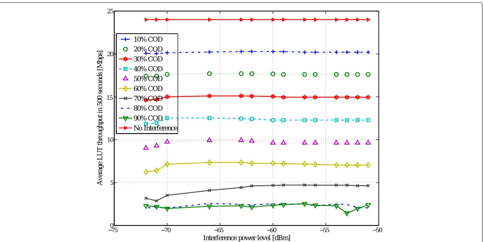
The second measurement studies the influence of chan-nel occupancy degree of the interference link on the throughput of the link under test. This measurement consists of 140 interference cases each characterized by a varying COD (10 levels) and a varying generated inter-ference level (14 levels) at node 19 (caused by interfering node 30). The COD was varied from 10% to 100% in 10% steps. For each channel occupancy degree, 14 different interference power levels (dBm) were observed at node 19: [-51,-52,-53,-54,-56,-57,-59,-60,-62,-63,-66,-70,-71, -72]. The data generation rate and transmit rate of the LUT were both set to 54 Mbps (COD = 100%). The transmit rate of the interfering link was set to 2 Mbps and was operated on channel 6, the same channel as the LUT. The value ofnwas set to 500 s.
Figure 6 shows the achieved average throughput (T) in 500 s for interference with varying channel occu-pancy degrees and with different interference power lev-els. As apparent from the figure, power levels do not play a key role in affecting the throughput. Analyzing the measurement results of the channel occupancy experi-ments implies an increasing nonlinear monotonic relation between the channel occupancy degree for COD values
below 80%. This relation can be expressed by the model below
T(CODIntf.)=ae−b.CODIntf.u(80−CODIntf.)
+a−b∗80u(CODIntf.−80),
(2)
where a = 24.5,b = −0.023, and CODIntf. denote the
interference COD. This model has aR2value of 0.97 and a root mean square error (RMSE) value of 1.18 Mbps. This fit has been calculated for throughput samples that are averaged over all interference power levels for every interference COD value. The statistics show an accept-able agreement between the model and the measurements which is also shown in Figure 7.
Channel occupancy degree indicates how the user is occupying the channel in time. Therefore, this met-ric can easily be calculated if the packet sniffer pro-vides information on the transmission rate of the sniffed packets.
3.4 Measurement III: influence of the interference TxRate on the throughput
In the third interference measurement, the influence of interference transmit rate on the throughput over the link under test was assessed. This measurement con-sists of 98 interference cases each characterized by a varying interference transmit rate and a varying gen-erated interference level (14 levels) at node 19 (caused by interfering node 30). The interference transmit rate
Figure 7Sample points and fitted values for measurement II.Each point is an averaged value of the throughput measurement with a single interference COD value and the various interference power levels of Figure 6.
was set to the values of [2,11,18,24,36,48,54] Mbps. For each interference transmit rate, 14 different inter-ference power levels (dBm) were observed at node 19: [-51,-52,-53,-54,-56,-57,-59,-60,-62,-63,-66,-70,-71, -72]. The data generation rate and transmit rate of the LUT were both set to 54 Mbps. The interfering link was
operating on channel 6, the same channel as the LUT. The interference COD is always 100% in this measure-ment. The value of n in this measurement is set to 10 s.
The measurement results in Figure 8 show a monotonic relation between the throughput and the interference
transmission rate. Equation 3 models the behavior by an exponential polynomial:
T(TxRateIntf.)=ced.TxRateIntf.+feg.TxRateIntf., (3)
wherec=9.001,d=0.004,f = −9.344,g= −0.083, and TxRateIntf.denote interference TxRate (see Figure 8). This
fit has anR2value of 0.9952 and an RMSE value of 0.3544
Mbps which is highly accurate.
3.5 Measurement IV: joint assessment of the interference TxRate and interference COD influence on the throughput
In measurements II and III, we assessed the influence of interference COD and TxRate on throughput by fixing one and varying the other parameter. This was a useful simpli-fication to understand how throughput changes with any of those parameters. Since interference COD and interfer-ence TxRate are not completely uncorrelated parameters, deriving a decent two-dimensional model requires joint assessment of the two parameters influence on through-put. Here, link L3 serves as LUT and the same selection of interference link as described in previous measurements is used. We measure the average achievable throughput in a 10-s interval with interference TxRates of [2, 11, 18, 24, 36, 48, 54] and interference COD values starting from 0% to 100% in steps of 6.25% resulting in a total of 105 measurement cases. All links are set to channel 6, and the transmit power of all terminals is set to 20 dBm. The TxRate of the LUT is set to 54 Mbps, and its COD is set to 100% percent such that the maximum achievable throughput is measured. The value of n is again 10 s.
Sample points in Figure 9 show the results of the mea-surement. Looking at the results of this measurement unveils the dependency of the interference COD and TxRate when predicting the throughput value. This is further investigated in the next section.
4 Development of the model
Data transmission rate of the Wi-Fi interface and the user activity are the key parameters that determine the spectrum utilization by any terminal. For a fixed amount of data transmission, higher transmission rate (TxRate) means less spectrum occupancy in time. Hence, an active user with low transmission rate occupies the spectrum to an extent that users of the other networks in the vicinity experience a much lower than expected throughput.
The model predicts the achievable throughput (T) based on the interference characteristics. The parame-ters that characterize the interference are the following: COD of the interference, interference TxRate, and inter-ference frequency channel. All parameters are obtainable using the monitor mode of IEEE 802.11 interfaces [24]
and packet tracing applications like libtrace [26] and tcp-dump [27]. Extension to all Wi-Fi channels is feasible by periodic monitoring of all channels or by exploiting more WLAN interfaces at different locations of the network each operating on a single channel.
Due to the dependency of the interference parameters, deriving a decent two-dimensional model to predict the throughput is crucial.
From the results of measurements II and III, we know that there is an exponential behavior between the throughput (T) and interference parameters COD and TxRate when the interference is on the same channel as the LUT. The investigation of the throughput behavior in sample points of Figure 9 shows that depending on the interference TxRate, the achieved throughput increases exponentially below a certain interference COD thresh-old. Therefore, by applying unit step function to the exponential models and partitioning the parameters space into linear and exponential regions, we come up with an accurate model. This is evidenced by the results of our suggested model in Equation 4 below:
T(CODIntf., TxRateIntf.)
where u(t) is the unit step function, TxRateIntf. denotes
interference TxRate, CODIntf.denotes interference COD,
and the coefficient parameters should be optimized for the intended link and the intended channel. The nonlin-ear least square optimization results for measurements on link L3 assign an a0 value of 23.23, b = 0.02 and
r = 0.5. These values are obtained by exploiting all the sample points of measurement IV. Figure 9 illustrates this realization of the model for sample points of link L3.The results of measurement IV show that the threshold of the aforementioned throughput exponential behavior decreases linearly from a COD of 90% for the TxRate of 2 Mbps up to the COD value of 60% for the TxRate of 54 Mbps. Inspired by this behavior, configuration of the step function arguments are optimized by a script that auto-matically investigates different combinations of the slope (r) and the intercept from a limited interval so that the least square error is achieved. The obtained R2 value is 0.9425 and the RMSE value is 1.34 which show the accu-racy of the model when used for the same link it was designed for. In the next section, we will show how the model is used inside the CDE and present its validation measurements.
Figure 9The 3D demonstration of the throughput model realized on link L3.
Figure 10 shows the RMSE andR2of the model realized with varying number of sample points. Every realization is a set of measurements with all possible TxRateIntf.
val-ues and CODIntf.values uniformly distributed between 0%
and 100%. TheR2value is always more than 0.94 and the RMSE is always less than 1.35 Mbps. These statistics show that the model can be devised with 42 samples.
5 Validation and integration of the model to the framework
In this section, we will show how the model developed in Section 4 will be used as the kernel of the cognitive decision engine. We will first explain how the input argu-ments of the model are prepared by the REM and will then describe how the CDE steers the network to the
optimal configuration set. We will also present the val-idation measurements configuration and results in this section.
5.1 Monitoring of wireless environment
The integration of this physical model into a CDE requires measurement of its input arguments, CODIntf.,
and TxRateIntf.. There are two possibilities to perform
measurements over the whole Wi-Fi spectrum; either by utilizing a number of additional Wi-Fi terminals on the monitor mode each operating on a different Wi-Fi channel simultaneously or having the terminal sweep the chan-nels periodically. In our implementation, we have used dedicated Wi-Fi interfaces as monitoring agents for every channel. The interfaces are brought up to the monitor mode of the IEEE 802.11 standard [24] to accept all ongo-ing detectable packets. A packet sniffer application [26] is then executed to capture all packets. The radio tap header [24] of every received packet provides crucial physical and link layer parameters such as the RSSI, packet length, and transmission rate of the packet. We propose to calculate the input arguments of the model of equation 4 by first calculating the equivalent interference transmission rate:
TxRateeq.(Mbps)=
whereN is the total number of packets sniffed,Riis the transmission rate of the sniffed packet,Liis the length of the sniffed packet, andLT is the total length of all sniffed packets in the current block of sniffed packets. Hav-ing the TxRateeq. calculated, we will find the equivalent
interference COD by
Using these relations, we can characterize the interfer-ence originating from several sources and give final values to the CDE for decision making. We should note that the COD estimations are accurate only if the sniffer cap-tures the whole present Wi-Fi traffic without dropping any packets which is the case in our measurements. For cop-ing with high data rates, we ensured zero packet drop by optimizing the script that was handling the tcpdump. This is realized by enlarging the tcpdump input buffer and ded-icating more computational power to the corresponding process.
5.2 Decision making
Whenever a decision is requested from the CDE, it queries the REM for values of CODIntf. and TxRateIntf. for each
channel. Once the inputs are ready, the CDE invokes the model on the channels with available inputs. The result
is a vector of throughput estimations for every chan-nel. Choosing the channel with the highest throughput value ignores the interference of overlapping channels. Therefore, if interference channels overlap with the mon-itored channels, the CDE should follow a rule-of-thumb approach where it takes into account both estimated throughput and the least interference influence from neighboring channels. The influence of interference from neighboring channels can be formulated by the results of measurement I, i.e., the CDE selects the channel with the least interference power level and the highest interference TxRate.
5.3 Model validation measurements
The objective of these measurements is to verify the two-dimensional model of Equation 4 for different sender-receiver distances, different link locations, different inter-ference power levels, and different number of interinter-ference links. To this end, different combinations of LUT ter-minals with various distances of sender-receiver were used in combination with various number of interfer-ence links. The links used as LUT are illustrated in Figure 4: links L2 and L4 are replications of L1 and L3, respectively, at other locations. L5 and L6 are other links used as LUT in these measurements. There are also three interference links IL1, Il2, and IL3 evenly spaced among the testbed (see Figure 4). When there is more than one interference link present, the sniffer derives the TxRateIntf.,eq.and CODIntf.,eq.by using Equations 5 and 6,
respectively.
For each location of the LUT, we investigate three cases for validating the model by utilizing one, two, and three interference sources simultaneously operating on the same channel of LUT. Each case is repeated with an interference transmission power of [0,10,14,20] dBm where we measure the average achievable throughput in a 10-s interval with interference TxRates of [2, 11, 18, 24, 36, 48, 54] and interference COD values starting from 0% to 100% in steps of 6.25%. All links are set to channel 6 and the transmit power of all terminals is set to 20 dBm. The TxRate of the LUT is set to 54 Mbps and its COD is set to 100% such that the maximum achievable throughput is measured.
5.4 Validation results
The model obtained by using measurements at link L3 is assessed with measurements on links L1, L2, L4, L5, and L6.
• The results of measurements with a single interference link are listed in Table 2.
Table 2 Statistics of the verifying measurements with one interference link
LUT Interference link R2 RMSE Maximum deviation
(Mbps) (Mbps)
The maximum deviation values of 2.9 Mbps for sin-gle interference link (Table 2) and 4.3 Mbps for multiple interference link (Table 3) might seem not ideal but hav-ing allR2values above 0.83 and the RMSEs not exceeding 1.9 Mbps. The CDE would safely use this model for com-paring the performance of the link on different channels. One should be cautious that the objective of the CDE is to optimize the throughput rather than accurately esti-mating it. Hence, the model optimized for a single link location can serve to predict the throughput at other links. This measurement setup was limited to the line-of-sight node locations and open environment propagation char-acteristics of the testbed. The tolerance of the model to location variability of the interference within the line-of-sight environment is a good incentive to use it for similar environments like home and conference halls where the dominant propagation channel is line-of-sight. However, measurements to support this extension is the subject for future research. One the other hand, for environments with more diverse propagation characteristics and larger sender-receiver distances, the same methodology could be used to derive appropriate models for each type of environment.
6 Proof of concept
We investigate two scenarios in this proof of concept to show the relevance of integrating the physical through-put model into the CDE and also the efficiency of using the proposed framework to tackle interference and bring
Table 3 Statistics of the verifying measurements with more than one interference link
LUT Interference link R2 RMSE Maximum deviation
(Mbps) (Mbps)
L5 IL1,IL2 0.89 1.46 2.61
L6 IL1,IL2 0.83 1.83 4.3
L5 IL1,IL2,IL3 0.83 1.62 + 2.9
L6 IL1,IL2,IL3 0.84 1.83 2.7
added value to the wireless network. In the first sce-nario, the CDE is used in a simplistic interference con-dition where interference characteristics are static, i.e., the CODIntf.,eq.and TxRateIntf.,eq.are stationary on every
channel. In the second scenario, the interference charac-teristics on all channels are varied over time.
6.1 Static interference
As a static interference proof of concept, we will investi-gate the scenario consisting of three interference sources operating simultaneously on non-overlapping Wi-Fi chan-nels 1, 6, and 11 each with a different COD and TxRate. Table 4 shows the interference profile of each source. For simplicity, in this proof of concept the CDE only seeks 2.4-GHz non-overlapping channels. The LUT is located on L3 (see Figure 4). The second Wi-Fi interface of the LUT transmitter scans the non-overlapping channels sequen-tially and quantifies the COD and TxRate of the interfer-ence on each channel. The CDE has to find the channel with the highest throughput estimation (Test.) based on
the proposed model. We also measured average through-put of LUT (Tactual) for each of the channels. The results
are all listed in Table 4.
The LUT was initially operating on channel 1. The results show that if there was no CDE, the LUT had to survive with a throughput of 2.45 Mbps. This scenario shows that the CDE can steer the network to a better sta-tus by estimating the throughput on other channels. As such, by changing towards the channel proposed by the CDE (channel 11) the LUT can achieve a throughput of 10.9 Mbps which shows a 344% improvement. The results of this proof of concept also show the accuracy of the proposed model in estimating the throughput.
6.2 Time variant interference
In this section, we investigate a scenario with time variant interference profiles. The interference is varied over time by periodically changing the interference profile of each channel. At the beginning of each interval, the ence profile is varied by changing the number of interfer-ence links and their corresponding COD and TxRate on each channel and it is fixed until the end of the interval. We assume that only IEEE 802.11g channels 1 and 6 are available. The duration of the interval should be selected
Table 4 Characteristics of the interference sources and the estimated and actual achieved throughputs (Test.and
Tactual, respectively)
Channel COD (%) TxRate (Mbps) Test.(Mbps) Tactual(Mbps)
1 75 2 2.68 2.45
6 55 18 4.73 4.98
such that the sniffer would be capable of characterizing the interference on all the intended channels.
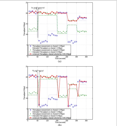
The duration of each interval in this scenario is set to 60 s firstly to ensure proper interference characterization and secondly to balance the interference dynamism. At the end of each interval, the CDE uses the collected information to steer the channel of LUT in order to optimize its through-put. The transition time depends majorly on the duration of the sniffing process. Lower sniffer intervals maintain smoother operation of the CDE. However, they are likely to lose interference profile changes if they are placed on the edge of profile change. We have used the CDE with two sniffer durations of 5 and 10 s. Table 5 shows the inter-ference profile of each interval on each of the channels. In the first three intervals (0 to 180 s), there is a single inter-ference link on any of the channels. During the intervals from 181 to 300 s, on one of the channels, there is inter-ference from two links. In the last interval (301 to 360 s), channel 1 has interference from three interfering links and channel 6 has a single interfering link. For intervals in Table 5 where there is more than one interference link, the equivalent interference configuration is listed before indi-vidual link configurations in brackets. The LUT is located on L5 (see Figure 4). The second Wi-Fi interface of the LUT transmitter scans the channels 1 and 6 sequentially. The CDE has to find the channel with the highest through-put estimation (Test.) based on the proposed model. We
also measured average throughput of LUT (Tactual) in a
separate measurement with the same interference profiles but without using the CDE to switch the channel of the LUT.
The results of the throughput measurements as well as the throughput estimations of the model are presented in Figure 11 for sniff interval of 5 s (Figure 11a) and 10 s (Figure 11b). This scenario shows that the CDE can steer the network to a better status by estimating the through-put on other channels. Depending on the sniffer interval, there might be transitional spikes in the CDE performance which could be solved by decreasing the sniffing period. As such, by changing towards the channel proposed by the CDE, the LUT can achieve an average throughput gain
of 183% and 70% compared to the case where it was con-stantly on channels 1 and 6, respectively. Figure 11 also shows that the throughput estimations follow the actual achieved throughput values on any of the channels despite the slight variations from the achieved throughput levels in intervals 120 to 180 and 240 to 300 which are neverthe-less below the maximum deviation values obtained in the validation measurements in Section 5.4.
6.3 Discussion on the limitations
Firstly, the model is developed in a pseudo-shielded all line-of-sight single-hop environment where the measure-ments were performed. The hidden node problem is not taken into consideration since it is not an issue in this environment. More precisely, the model does not con-sider interference of nodes that are not in the radio range of the sniffers. The sniffers are assumed to capture all present traffic without dropping any packets. If for any reason (other ISM band interference such as Bluetooth, microwave ovens, and ZigBee) the interference is not per-ceived by the sniffers, the event detector of the CDE (see Figure 3) assists by detecting the unpredicted throughput degradation in the network.
Secondly, the physical model is developed for UDP traf-fic since its objective was to find the maximum capacity of the channel given a certain interference profile. If the application requires a reliable end-to-end connection, the same methodology we have incorporated in this paper shall be used to create a model which accounts for TCP traffic.
Thirdly, deploying both the CDE and the REM imposes data and processing overhead on the network. Spectrum monitoring data overhead could be formulated in two cases depending on the mobility of spectrum sensing devices. For a distributed spectrum sensing which col-lects information from fixed and mobile terminals, the data overhead to update the REM would scale with the number of mobile terminals and update the frequency of the REM. Excluding mobile devices from spectrum mon-itoring and only depending on the fixed Wi-Fi sniffers do not introduce any data overhead to the wireless network.
Table 5 Characteristics of the interference sources during each interval
Channel 1 Channel 6
Interval Interference links CODeq. TxRateeq. Interference links CODeq. TxRateeq.
(a)
10s sniff interval
(b)
Figure 11Comparison of throughput on channels 1 and 6 with and without using the CDE.With sniff intervals of(a)5 s and(b)10 s.
Event detection also imposes data overhead to the wire-less network which would be negligible short-length data packets in the order of a few bytes for each event.
7 Application outlook of the framework
The goal of this section is to showcase the usefulness of the REMs and the proposed methodology in this cog-nitive framework when it is used for optimizing either
the interference profile, i.e., traffic characteristic of the interference, is adjustable.
When the user initiates the scenario, the audio/iperf stream server starts to transmit multicast audio/iperf traf-fic with an initial set of traftraf-fic configurations. If the target QoS metric is audio quality, at the same time, all clients will translate their received network characteristics (throughput, delay, and jitter) into audio MOS scores (in a scale of 1 to 5, where 1 corresponds to the poorest qual-ity and 5 to the highest) and store the result in the DB. The MOS value is calculated by the E Model proposed by the ITU G.107 recommendation [22]. The REM will then illustrate the interpolated map of the MOS/throughput and other relevant parameters and feeds the necessary arguments to the CDE.
Due to the fundamental throughput-delay trade off [28], selecting the channel with the highest throughput estima-tion does not necessarily guarantee the lowest delay or jitter. Consequently, for audio quality target metric, the CDE should therefore use a different model that estimates the MOS value based on the estimated throughput and reported delay and jitter from the REM on each chan-nel. In this way, the CDE estimates the MOS values on each channel and determines corrective actions that must be implemented on the NUT for the next round of audio streaming. Figure 12 is an example of REMs for RSSI and MOS values. Each map illustrates its corresponding parameter alongside the location of the network elements. Clients that are closer to the sender indicate higher RSSI values and consequently bring about higher MOS values to their users.
When the corrective actions have been implemented and the MOS/throughput have been illustrated by the
REM, we need to assess the efficiency of corrective actions, i.e., how much the network is performing better in terms of the intended metric (MOS/throughput). To address this, we define the objective of the scenario in the next paragraph.
The optimal configuration set of the network (node locations and all the parameters mentioned earlier) is achieved when∀i∈NUT(QoSi≥QoS0). In this formula, QoSirefers to the QoS value of theith client of NUT and QoS0is a certain threshold. This scenario will follow the following steps in order to showcase the advantages of the REM and the CDEs.
1. All clients are set to the default (initial) configuration set.
2. While there is no interference in the environment, the NUT starts the first round of audio/iperf stream and all the clients record their MOS/throughput. 3. Based on the results of the previous round, the REM
represents the QoS values and the CDE will optimize the configuration set by means of the corrective actions.
4. The interference network is set to its default profile. The interference stream starts here.
5. While there is interference on the air, the NUT starts another round of audio/iperf streaming. As before, all clients keep track of the QoS values.
6. At this step, the REM and/or the CDE should quantify the added value of the corrective actions in terms ofMOS, throughput, energy, etc.
7. If the objective is achieved, the iteration will stop; otherwise, CDE implements corrective actions to the NUT and the iteration starts again from 4.
(a)
(b)
This is a very simple example of how the models can be used. Future research will comprise the development of physical models for audio/video QoS metrics and a CDE based on the corresponding models.
8 Conclusion and future work
A novel framework for cognitive wireless networking is proposed in this paper. The framework comprises differ-ent elemdiffer-ents. REMs and the cognitive decision engine are the most integral parts of the framework to char-acterize the radio environment and make appropriate decisions reactively to the environment dynamism. Based upon numerous exploratory measurements, a novel physi-cal throughput model accounting for interference channel occupancy degree and interference transmission rate was devised and verified in a pseudo-shielded testlab environ-ment. The model was implemented within the CDE. The framework was applied to realistic stationary and time-variant interference scenarios where an average through-put gain of 344% was gained in the stationary interference scenario and 70% to 183% was gained in the time-variant interference scenario.
Future research on this framework includes compari-son of the performance of the CDE based on the pro-posed model with smarter higher level algorithms and the integration of this type of physical modeling with other decision algorithms to achieve more efficient algo-rithms. The physical model was developed in a pseudo-shielded line-of-sight environment; therefore, on the one hand, extension to other line-of-sight environments like home or conference halls should be investigated, and on the other hand, incorporating the same methodology to develop similar models for other types of environments would be the topic of further research.
Competing interests
The authors declare that they have no competing interests.
Authors’ contributions
MP executed all measurements and drafted the manuscript in collaboration with DP, WJ, and LM. DD, KC,and TD contributed partially to the radio environment maps by optimizing the IDW interpolation technique. WL and IM participated in the development of the passive packet sniffer. ET contributed in formulating the physical model and its statistical assessment. All authors read and approved the final manuscript.
Acknowledgements
This work was supported by the iMinds-ICON QoCON project, co-funded by iMinds, a research institute founded by the Flemish Government in 2004, and the involved companies and institutions. DD is a Post-Doctoral Fellow of the FWO-V (Research Foundation - Flanders). The research is also partly funded by the Fund for Scientific Research - Flanders (FWO-V, Belgium) project G.0325.11N.
Received: 26 May 2014 Accepted: 29 October 2014 Published: 15 November 2014
References
1. IJ Mitola, JGQ Maguire, Cognitive radio: making software radios more personal. IEEE Pers. Commun.6(4), 13–18 (1999). doi:10.1109/98.788210
2. D Plets, M Pakparvar, W Joseph, L Martens, inProceedings of the IEEE International Symposium on Broadband Multimedia Systems and
Broadcasting (BMSB). Influence of intra-network interference on quality of
service in wireless LANs (London, UK, 5–7 June 2013)
3. S Bouckaert, P Becue, B Vermeulen, B Jooris, I Moerman, P Demeester, in
Proceedings of TridentCom. Federating wired and wireless test facilities
through Emulab and OMF: the iLab.t use case (Thessaloniki, Greece, 11–13 June 2012)
4. Y Zhao, Enabling cognitive radios through radio environment maps. PhD thesis, Virginia Polytechnic Institute and State University, Blacksburg, Virginia (May 2007). http://scholar.lib.vt.edu/theses/available/etd-05212007-162735/. Accessed 28 June 2013
5. J Riihijarvi, P Mahonen, M Wellens, M Gordziel, inIEEE 19th International
Symposium on Personal, Indoor and Mobile Radio Communications (PIMRC).
Characterization and modelling of spectrum for dynamic spectrum access with spatial statistics and random fields (Cannes, France, 15–18 Sept 2008), pp. 1–6. doi:10.1109/PIMRC.2008.4699912
6. S-J Kim, E Dall’Anese, G Giannakis, Cooperative spectrum sensing for cognitive radios using Kriged Kalman filtering. IEEE J. Selected Topics Signal Process.5, 24–36 (2011)
7. M Portoles-Comeras, C Ibars, J Nunez-Martinez, J Mangues-Bafalluy, in
2011 IEEE Vehicular Technology Conference (VTC Fall). Characterizing WLAN
medium utilization for radio environment maps (San Francisco, CA, USA, 5–8 Sept 2011), pp. 1–5. doi:10.1109/VETECF.2011.6093284
8. J van de Beek, E Lidstrom, T Cai, Y Xie, V Rakovic, V Atanasovski, L Gavrilovska, J Riihijarvi, P Mahonen, A Dejonghe, P Van Wesemael, M Desmet, inIEEE International Symposium on Dynamic Spectrum Access
Networks (DYSPAN). REM-enabled opportunistic, LTE in the TV band
(Bellevue, WA, USA, 16–19 Oct 2012), pp. 272–273. doi:10.1109/DYSPAN.2012.6478140
9. M Hasegawa, H-N Tran, G Miyamoto, Y Murata, S Kato, inIEEE 18th International Symposium on Personal, Indoor and Mobile Radio
Communications (PIMRC). Distributed optimization based on
neurodynamics for cognitive wireless clouds (Athens, Greece, 3–7 Sept 2007), pp. 1–5. doi:10.1109/PIMRC.2007.4394658
10. Z Zhang, X Xie, inITI 5th International Conference on Information and
Communications Technology (ICICT). Intelligent cognitive radio: research
on learning and evaluation of CR based on neural network (Cairo, Egypt, 16–18 Dec 2007), pp. 33–37. doi:10.1109/ITICT.2007.4475612
11. N Baldo, M Zorzi, in5th IEEE Consumer Communications and Networking
Conference (CCNC). Learning and adaptation in cognitive radios using
neural networks (Las Vegas, NV, USA, 10–12 Jan 2008), pp. 998–1003. doi:10.1109/ccnc08.2007.229
12. C Blum, A Roli, Metaheuristics in combinatorial optimization: overview and conceptual comparison. ACM Comput. Surv.35(3), 268–308 (2003). doi:10.1145/937503.937505
13. D Thilakawardana, K Moessner, in2nd International Conference on Cognitive
Radio Oriented Wireless Networks and Communications (CrownCom). A
genetic approach to cell-by-cell dynamic spectrum allocation for optimising spectral efficiency in wireless mobile systems (Orlando, FL, USA, 1–3 Aug 2007), pp. 367–372. doi:10.1109/CROWNCOM.2007.4549825 14. JM Kim, SH Sohn, N Han, G Zheng, YM Kim, JK Lee, in3rd International
Conference on Cognitive Radio Oriented Wireless Networks and
Communications (CrownCom). Cognitive radio software testbed using
dual optimization in genetic algorithm (Singapore, 15–17 May 2008), pp. 1–6. doi:10.1109/CROWNCOM.2008.4562484
15. J De Bruyne, W Joseph, L Verloock, C Olivier, W De Ketelaere, L Martens, Field measurements performance analysis of an 802.16 system in a suburban environment. Wireless Commun. IEEE Trans.8(3), 1424–1434 (2009). doi:10.1109/TWC.2009.080085
16. W-Y Lee, IF Akyldiz, A spectrum decision framework for cognitive radio networks. Mobile Comput. IEEE Trans.10(2), 161–174 (2011). doi:10.1109/TMC.2010.147
17. IEEE,IEEE Std 802.22-2012: IEEE Recommended Practice for Information Technology-Telecommunications and Information Exchange Between Systems Wireless Regional Area Networks (WRAN)—Specific Requirements
Part 22.2: Installation and Deployment of IEEE 802.22TMSystems.
(IEEE, Piscataway, 2012)
Commun. Netw.2013(1), 228 (2013). doi:10.1186/1687-1499-2013-228. Accessed 26 May 2014
19. D Shepard, inProceedings of the 1968 23rd ACM National Conference. A two-dimensional interpolation function for irregularly-spaced data (Las Vegas, NV, USA, 27–29 Aug 1968), pp. 517–524.
doi:10.1145/800186.810616
20. D Plets, W Joseph, K Vanhecke, E Tanghe, L Martens, Coverage prediction and optimization algorithms for indoor environments. EURASIP J. Wireless Commun. Netw.2012(1), 1–23 (2012). doi:10.1186/1687-1499-2012-123 21. Information Sciences Institute, University of Southern California,RFC 791:
Internet Protocol. (University of Southern California, Los Angeles, 1981)
22. ITU-T Study Group 12,ITU-T Recommendation G.107. International Telephone Connection and Circuits. General Definitions, The E model, a
Computational Model for Use in Transmission Planning, (2014). International
Telecommunication Union. http://handle.itu.int/11.1002/1000/12120 23. Iperf, The TCP/UDP bandwidth measurement tool. http://iperf.fr/.
Accessed 19 July 2013
24. IEEE, IEEE Std 802.11-2012: IEEE Standard for Information
Technology-Telecommunications and Information Exchange Between Systems Local and Metropolitan Area Networks?Specific Requirements part 11: Wireless LAN Medium Access Control (MAC) and Physical Layer (PHY) Specifications (Revision of IEEE Std 802.11-2007), 1–2793 (2012). doi:10.1109/IEEESTD.2012.6178212
25. M Heusse, F Rousseau, G Berger-Sabbatel, A Duda, inTwenty-Second
Annual Joint Conference of the IEEE Computer and Communications.
Performance anomaly of 802.11b, vol. 2 (San Francisco, CA, USA, 30 March–3 April 2003), pp. 836–8432. doi:10.1109/INFCOM.2003.1208921 26. S Alcock, P Lorier, R Nelson, inACM SIGCOMM Computer Communication
Review. Libtrace: a packet capture and analysis library, vol. 42 2, (March
2012), pp. 42–48. doi:10.1145/2185376.2185382
27. Tcpdump/Libpcap, tcpdump: a powerful command-line packet analyzer. http://www.tcpdump.org/. Accessed 19 July 2013 28. AE Gamal, J Mammen, B Prabhakar, D Shah, Throughput-delay
trade-off in wireless networks. INFOCOM.1, 475 (2004). doi:10.1109/INFCOM.2004.1354518
doi:10.1186/1687-1499-2014-191
Cite this article as:Pakparvaret al.:A cognitive QoS management framework for WLANs.EURASIP Journal on Wireless Communications and
Networking20142014:191.
Submit your manuscript to a
journal and benefi t from:
7Convenient online submission 7Rigorous peer review
7Immediate publication on acceptance 7Open access: articles freely available online 7High visibility within the fi eld
7Retaining the copyright to your article