R E S E A R C H
Open Access
Dynamical analysis of almost periodic
solution for a multispecies predator-prey
model with mutual interference and time
delays
Qin Liu, Yuanfu Shao
*, Si Zhou, Zhen Wang and Hairu Chen
*Correspondence:
School of Science, Guilin University of Technology, Guilin, Guangxi 541004, P.R. China
Abstract
In this paper, we build a multispecies predator-prey model with mutual interference and time delays. By means of the comparison theorem, Ascoli theorem and Lebesgue dominated convergence theorem, we establish the sufficient conditions of
permanence and investigate the existence of a unique almost periodic solution. By constructing a suitable Lyapunov function, we obtain that the positive almost periodic solution is globally attractive. Finally, we give numerical simulations to indicate the complex dynamical behaviors of this system.
Keywords: almost periodic solution; global attractivity; mutual interference; numerical simulation
1 Introduction
In population dynamics, the linkages between predator and prey are usually expressed by different functional response functions, which reflect different dynamical behaviors. Holling [1] carried out a large number of experiments on predator and prey and got some different functional response functions. For example, the mathematical expression of Hollingxi(i= 1, 2) model is as follows [2]:
(X) = αX 2
β2+X2.
Besides, in ecosystems, mutual interference between species is always present. The au-thors [3] proposed a mutual interference factor that tended to leave when the host or parasite met. A lot of articles studied the ecosystem with interference factors. Their ob-tained results showed that the effect of this factor should not be ignored [4–7]. For ex-ample, Wang et al. [6] concluded that mutual interference had great effect on the relative properties of predator-prey models.
In real life, time delay always exists. Food digestion time, resource regeneration time, mature time, pregnancy period and so on, these all can be expressed by time delay. Usu-ally time delay plays a key role in many systems. For example, time delay can destroy the
stability of the positive equilibrium. The obtained results showed that delayed differential equations exhibited more complex dynamical properties than ordinary differential equa-tions [8–14]. Du et al. [10] gave the following model:
⎧ ⎨ ⎩ ˙
x=x(t)(r1(t) –b1(t)x(t–τ(t))) –c1(t)x 2(t)
x2(t)+k2ym(t), ˙
y=y(t)(–r2(t) –b2(t)y(t)) +c2(t)x 2(t)
x2(t)+k2ym(t),
(1.1)
where all parameter meanings can be seen in [10]. The time delay of system (1.1) made the system very unstable and led to more complex dynamical behaviors. At the same time, the research methods were also very different from other systems.
From the point of view of the interaction between biology and environment, Darwin thought that biological variation, heredity and natural selection could lead to the adaptive change of organisms. We know that natural environment is not a constant, and organisms can change their habits to adapt to the new environment, which is called adaptive con-trol. In recent years, adaptive control has been widely used in biological control systems, aerospace systems, satellite tracking systems, and so on [15, 16].
On the other hand, in Ref. [10], the authors assume that the coefficientsr1(t),b1(t),τ(t),
c1(t),r2(t),b2(t),c2(t) of system (1.1) are continuous positive almost periodic functions. It is well known that the assumption of almost periodicity of the coefficients in (1.1) is a way of incorporating the time-dependent variability of the environment, especially when the factors of the environment exhibit periodical changes with not necessarily commensurate periods, such as weather, food, mating habits, harvest, etc. In view of these factors, it is necessary to study the relevant properties of ecosystems by using almost periodic coeffi-cients. Recently, many scholars have studied the almost periodic solution and got some nice results, which showed that the almost periodic solution of a population dynamical system with mutual interference and time delay had wider application value [10, 17–19].
However, in the actual ecosystem, predator and prey always coexist, which is a common and widespread phenomenon. The dynamical property of a multispecies predator-prey system is much more complex than the system with only two or three species, and the analytical methods are very different [11, 20–22].
Based on the above discussion, we establish a multispecies predator-prey model with al-most periodic coefficients, mutual interference and time delays. The corresponding math-ematical model is as follows:
⎧ ⎪ ⎪ ⎪ ⎪ ⎪ ⎪ ⎨ ⎪ ⎪ ⎪ ⎪ ⎪ ⎪ ⎩
xi(t) =xi(t)[ri(t) –nk=1bik(t)xk(t–τk(t)) –mk=1
cik(t)xi(t) x2i(t)+fik(t)y
α k(t)],
i= 1, 2, . . . ,n,
yj(t) =yj(t)[–rj(t) –
m
k=1pjk(t)yk(t) +
n
k=1
qkj(t)x2k(t) x2k(t)+fkj(t)y
α–1
j (t)],
j= 1, 2, . . . ,m,
(1.2)
with the initial conditions
xi(χ) =φi(χ), yj(χ) =ψj(χ); φi(χ),ψj(χ)∈C
[–τ, 0],R+
,χ∈[–τ, 0], (1.3)
whereτ =maxt∈R{τk(t),k= 1, 2, . . . ,m},τk(t) is a nonnegative and continuously
Table 1 Notations used to denote parameters
Parameters Description
xi(t) The population of species of theith prey att.
yj(t) The population of species of theith predator att.
ri(t) The population growth of prey without predators.
rj(t) The decay rate of predator population without prey.
α The mutual interference of predator and 0 <α< 1.
bik(t) The number of prey decreased due to inter-specific competition.
pjk(t) The number of predator decreased due to inter-specific competition.
cik(t) The amount of prey eaten by predator.
qkj(t) Conversion of energy from prey to predators.
pjk(t),qkj(t),fkj(t) are all continuous positive almost periodic functions onRand the brief
description about other parameters used in system (1.2) is presented in Table 1.
In this article, we aim to investigate the dynamical properties of almost periodic system (1.2), which can greatly enrich the biological background.
The structure of the article as follows. In Section 2, we introduce several important defi-nitions and lemmas. We discuss the permanence of the system in Section 3. Next, we prove the global attractivity of system (1.2) in Section 4. In Section 5, we give conditions of the existence and uniqueness of almost periodic solutions for the system. We put numerical simulations in Section 6. In Section 7, we give a brief conclusion to this paper.
2 Main descriptions
In this part, we give some definitions and lemmas. For continuous and boundedf onR, we denotefu=sup
t∈Rf(t),fl=inft∈Rf(t).
Definition 2.1 The positive solution (x(t),y(t))T = (x
1(t),x2(t), . . . ,xn(t),y1(t),y2(t), . . . ,
ym(t))T of system (1.2) is said to be globally attractive if, for any other positive solution
(x¯(t),y¯(t))T= (x¯
1(t),x¯2(t), . . . ,x¯n(t),y¯1(t),y¯2(t), . . . ,y¯m(t))T of (1.2), the following condition
holds:
lim
t→+∞
n
i=1
xi(t) –x¯i(t)+ n
j=1
yj(t) –y¯j(t)
= 0.
Definition 2.2([23]) A functionf(t,x) is said to be almost periodic intuniformly with respect tox∈X iff(t,x) is continuous and, for∀ε> 0, it is possible to find a constant
I(ε) > 0 such that, for any interval of lengthI(ε), there existsτ such that
f(t+τ,x) –f(t,x)<ε,
where the numberτ is called anε-translation number off(t,x).
By the continuity of almost periodic functions, we obtain that the almost periodic coef-ficients satisfymini=1,2,...,n;j=1,2,...,m{rli,rjl,blik,pljk,cikl ,qlkj}> 0 andmaxi=1,2,...,n;j=1,2,...,m{rui,ruj,buik, pu
jk,cuik,qukj}< +∞. For, the characteristics and relevant definitions of almost periodic
Definition 2.3([25]) An almost periodic functionf :R→Ris said to be asymptotic if there exist an almost periodic functionq(t) and a continuous functionr(t) such that
f(t) =q(t) +r(t), r(t)→0 ast→ ∞.
Lemma 2.1([26]) If the function f(t)is nonnegative,integral and uniformly continuous on[0, +∞),thenlimt→∞f(t) = 0.
Then Lemma 2.2 is obtained.
Lemma 2.3([27]) Suppose that the continuous operator A maps the closed and bounded convex set Q⊂Rnonto itself,then the operator A has at least one fixed point in the set Q.
3 Permanence of system (1.2)
Theorem 3.1 If the following condition holds:
Proof By the first equation of (1.2), we get
xi(t)≤xi(t)ri(t). (3.1)
Integrating (3.1), we havexi(t)≤xi(t–τ)exp(riuτ),t>τ, that is,
xi(t–τ)≥xi(t)exp
–ruiτ, t>τ. (3.2)
Combining (3.2) and the first equation of (1.2), we have
xi(t)≤xi(t)
riu–bliixi(t)exp
–ruiτ, t>τ. (3.3)
By applying Lemma 2.4 to (3.3), we obtain
lim
t→+∞supxi(t)≤
ru i bl
iie–r u
iτ ≡Mi. (3.4)
By (3.4), there existsT1>τ, whent≥T1andT1→ ∞, then
xi(t)≤Mi. (3.5)
By (3.5), there also existsT2=T1+τ, whent≥T2, then
xi(t–τ)≤Mi. (3.6)
Combining (3.6) and the second equation of (1.2), we have
yj(t)≤yj(t)
n
k=1
qkju(t)yjα–1(t) –rlj(t)
≤yαj(t)
n
k=1
qukj(t) –rjl(t)y1–α(t)
, t≥T2. (3.7)
Using Lemma 2.5 to (3.7), then
yj(t)≤
n
k=1qukj(t) rlj(t) +
y1–α(0) –
n
k=1qukj(t) rjl(t)
e–rjl(t)(1–α)t
1
1–α
, ∀t≥0. (3.8)
Therefore, there existsT3> 0 such that
yj(t)≤
3n
k=1qukj(t)
2rlj
1
1–α
≡Nj, t>T3. (3.9)
Combining (3.5), (3.6), (3.9) and the first equation of (1.2), we get
xi(t)≥xi(t)
ril–
n
k=1,k=i
buik(t)Mk–buiixi
t–τi(t)
–
m
k=1
cu ikMiN
α k fl
ik
Supposexi(˜t) is any local minimal value ofxi(t), then we have
From (3.11) and (3.12), we have
xi
From (3.13) and (3.14), then
xi(˜t)≥ ˆ
It follows from Lemma 2.5 that there existsT6> 0 such that
yj(t)≥
Next, we prove that system (1.2) has at least one bounded positive solution fort≥0. Define ={(x(t),y(t))T = (x
1(t),x2(t), . . . ,xn(t),y1(t),y2(t), . . . ,ym(t))T ∈Rn+m|(x(t),y(t))T
is the solution of system (1.2), satisfyingmi≤xi(t)≤Mi,nj≤yj(t)≤Nj,t∈R}.
Theorem 3.2 For system(1.2),the set=∅.
Proof According to the characteristics of an almost periodic function, for a sequence of {tγ},tγ → ∞asγ → ∞, thenri(t+tγ)→ri(t),rj(t+tγ)→rj(t),bil(t+tγ)→bil(t),pjk(t+ tγ)→pjk(t),cik(t+tγ)→cik(t), qlj(t+tγ)→qlj(t), τi(t+tγ)→τi(t), fij(t+tγ)→fij(t)
(i,l= 1, 2, . . . ,n;j,k= 1, 2, . . . ,m) uniformly onRasγ → ∞. By Lemma 2.3, system (1.2) has at least one solutionz(t) = (x(t),y(t))Tsatisfyingm
i≤xi(t)≤Mi,nj≤yj(t)≤Njwhen t>T.
Obviously, the sequencez(t+tγ) is uniformly bounded and equi-continuous on any
bounded subset ofR. By the Ascoli theorem, we know there exists a subsequencez(t+tλ)
which converges to a continuous function
g(t) =g1(t),g2(t)
T
=g11(t),g21(t), . . . ,gn1(t),g12(t),g22(t), . . . ,gm2(t)
T
asλ→ ∞uniformly on any bounded subset ofR.
MakeT7∈R, supposeT7+tλ≥Tfor allλ. Whent≥0, we obtain
xi(t+tλ+T7) –xi(tλ+T7)
= t+T7
T7
xi(s+tλ) ri(s+tλ) – n
k=1
bik(s+tλ)xk
(s+tλ) –τk(s+tλ)
–
m
k=1
cik(s+tλ)xi(s+tλ) x2
i(s+tλ) +fik(s+tλ)
yαk(s+tλ)
ds, (3.17)
yj(t+tλ+T7) –yj(tλ+T7)
= t+T7
T7
yj(tλ+s) –rj(s+tλ) – m
k=1
pjk(s+tλ)yk(s+tλ)
+
n
k=1
qkj(s+tλ)x2k(s+tλ) x2
k(s+tλ) +fkj(s+tλ)
yαj–1(s+tλ)
ds. (3.18)
Lettingλ→ ∞in (3.17) and (3.18), for∀t≥0, by the Lebesgue dominated convergence theorem, we get
gi1(t+T7) –gi1(T7)
= t+T7
T7
gi1(s) ri(s) – n
k=1
bik(s)gk1
s–τk(s)
–
m
k=1
cik(s)gi1(s)
gi21(s) +fik(s) gαk2(s)
ds,
gj2(t+T7) –gj2(T7)
= t+T7
T7
gj2(s) –rj(s) – m
k=1
pjk(s)gk2(s) +
n
k=1
qkj(s)gk21(s)
g2
k1(s) +fkj(s)
gα–1
j2 (s)
ds.
It is easy to knowmi≤gi1(t)≤Mi,nj≤gj2(t)≤Njfor anyt∈R. Thus, the set=∅,
that is, system (1.2) has at least one bounded positive solution.
4 Global attractivity of system (1.2)
Theorem 4.1 If the parameters of system(1.2)satisfy condition [H1]and the following
conditions:
Next, we set up several Lyapunov functions. Let
Vi1(t) =lnx¯i(t) –lnxi(t). (4.2)
By calculating the upper right derivative ofVi1(t) along system (1.2), we have
–
Substituting (1.2) into (4.3), we get
Next, we define
Calculating its Dini derivative along system (1.2), we get
×
Define the Lyapunov functionalV(t) as follows:
Using Lemma 2.1, we get
lim
t→+∞
n
i=1
x¯i(t) –xi(t)+ m
j=1
y¯j(t) –yj(t)
= 0 and
lim
t→+∞x¯i(t) –xi(t)= 0, t→lim+∞y¯j(t) –yj(t)= 0.
(4.18)
Therefore, system (1.2) is globally attractive.
5 Existence of almost periodic solution
Theorem 5.1 Suppose[H1], [H2]and[H3]hold,then system(1.2)has a unique almost
periodic solution.
Proof From Theorem 3.2, we know (x(t),y(t))T,t∈Ris a bounded positive solution. Then
there exists a sequence{tλ},tλ→ ∞asλ→+∞such that (x(t+tλ),y(t+tλ))Tis a solution
of the following system (5.1): ⎧
⎪ ⎨ ⎪ ⎩
xi(t) =xi(t)[ri(t+tλ) –
n
k=1bik(t+tλ)xk(t–τk(t)) –
m
k=1
cik(t+tλ)xi(t) x2i(t)+fik(t+tλ)
yα k(t)],
yj(t) =yj(t)[–rj(t+tλ) –
m
k=1pjk(t+tλ)yk(t) +
n
k=1
qkj(t+tλ)x2k(t) x2
k(t)+fkj(t+tλ)
yαj–1(t)].
(5.1)
From the above and Theorem 3.1, we know (x(t+tλ),y(t+tλ))Tand (x(t+tλ),y(t+tλ))Tare
uniformly bounded. Clearly, the sequence (x(t+tλ),y(t+tλ))Tis equi-continuous. By the
Ascoli theorem, there exists a uniformly convergent subsequence{(x(t+tλ),y(t+tλ))T} ⊆
{(x(t+tλ),y(t+tλ))T}such that, for any∀ε> 0, there existsλ0(ε) > 0 with the property that ifλ, >λ0(ε), then
xi(t+t) –xi(t+tλ)<ε, yj(t+t) –yj(t+tλ)<ε,
which indicates that (x(t+tλ),y(t+tλ))T is an almost periodic and asymptotic function.
Then there exist functionsgi1(t),gj2(t),hi1(t),hj2(t) such that
xi(t) =gi1(t) +hi1(t), yj(t) =gj2(t) +hj2(t),
where
lim
λ→+∞gi1(t+tλ) =gi1(t), λ→lim+∞gj2(t+tλ) =gj2(t),
lim
λ→+∞hi1(t+tλ) = 0, λ→lim+∞hj2(t+tλ) = 0,
gi1(t),gj2(t) are almost periodic functions. It shows that
lim
λ→+∞xi(t+tλ) =gi1(t), λ→lim+∞yj(t+tλ) =gj2(t).
Besides, we still have
lim
λ→+∞x
i(t+tλ) = lim λ→+∞h→lim¯ 0
xi(t+tλ+h¯) –xi(t+tλ)
¯
h =h→lim¯ 0
gi1(t+h¯) –gi1(t)
¯
lim
λ→+∞y
j(t+tλ) = lim λ→+∞h→lim¯ 0
yj(t+tλ+h¯) –yj(t+tλ)
¯
h =h→lim¯ 0
gj2(t+h¯) –gj2(t)
¯
h . (5.3)
Therefore, the derivativesgi1(t),gj2(t) exist.
Next, we proveg(t) = (g1(t),g2(t))Tis an almost periodic solution of system (1.2). By the characteristics of almost periodic solution, there exists a sequence {tγ},tγ →
∞asγ →+∞such that ri(t+tγ)→ri(t),rj(t+tγ)→rj(t),bil(t+tγ)→bil(t),pjk(t+ tγ)→pjk(t),cik(t+tγ)→cik(t), qlj(t+tγ)→qlj(t), τi(t+tγ)→τi(t), fij(t+tγ)→fij(t)
(i,l= 1, 2, . . . ,n;j,k= 1, 2, . . . ,m) asγ → ∞uniformly onR. Obviously,limγ→+∞xi(t+tγ) = gi1(t),limγ→+∞yj(t+tγ) =gj2(t). So we have
gi1(t) = lim
γ→+∞x
i(t+tγ)
= lim
γ→+∞xi(t+tγ)
ri(t+tγ) – n
k=1
bik(t+tγ)xk
(t+tγ) –τk(t+tγ)
–
m
k=1
cik(t+tγ)xi(t+tγ)yαk(t+tγ) x2
i(t+tγ) +fik(t+tγ)
=gi1(t)
ri(t) – n
k=1
bik(t)gk1
t–τk(t)
–
m
k=1
cik(t)gi1(t)gkα2(t)
gi21(t) +fik(t)
,
gj2(t) = lim
γ→+∞y
j(t+tγ)
= lim
γ→+∞yj(t+tγ)
–rj(t+tγ) – m
k=1
pjk(t+tγ)xk
(t+tγ) –τk(t+tγ)
+
n
k=1
qik(t+tγ)x2k(t+tγ)yαk–1(t+tγ) x2
k(t+tγ) +fkj(t+tγ)
=gj2(t)
–rj(t) –
m
k=1
bik(t)gk2(t) +
n
k=1
qkj(t)g2k1(t)g α–1
k2 (t)
gk21(t) +fkj(t)
.
From the above, we knowg(t) satisfies (1.2), that is, it is a positive almost periodic solution. Next, we prove that the positive almost periodic solution of system (1.2) is unique. Letg(t) > 0 andg¯(t) > 0 be any two almost periodic solutions of system (1.2), then we claim thatg1(t)≡ ¯g1(t) andg2(t)≡ ¯g2(t) for∀t∈R. Otherwise, there is at least oneξ∈R such thatgi1(ξ)= g¯i1(ξ), that is,|gi1(ξ) –g¯i1(ξ)|:=δ> 0. Then
δ=gi1(ξ) –g¯i1(ξ)= lim
γ→+∞xi(ξ+tγ) –x¯i(ξ+tγ)=t→lim+∞xi(t) –x¯i(t)> 0,
which is a contradiction to (4.18). Thus∀t∈R,g1(t)≡ ¯g1(t) holds. By the same method,
we can prove that∀t∈R,g2(t)≡ ¯g2(t).
Remark 5.1 Ifτi(t)≡τi, whereτi(i= 1, 2, . . . ,n) is a nonnegative constant, then
Corollary 5.1 Makeτi(t)≡τi,whereτi≥0.If system(1.2)satisfies both[H1]and the
fol-lowing two conditions:
lim
then system(1.2)has a unique positive almost periodic solution which is globally attractive.
6 Model simulation
We give examples to verify the correctness of our theoretical results in this part.
Example 6.1 Consider the following system:
⎧
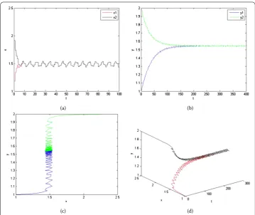
By calculation, the parameters of (6.1) meet the conditions of Theorem 3.1 and Corol-lary 5.1. Using MATLAB, by simulation, time series diagrams of (6.1) are shown in Fig-ure 1. FigFig-ure 1 indicates that (6.1) is persistent and has a unique positive almost periodic solution which is globally attractive.
In order to demonstrate the dynamical behaviors of a multispecies predator-prey sys-tem, we give the time series diagrams with only three species in system (1.2).
Example 6.2 Consider the following system:
(a) (b)
(c) (d)
Figure 1 (a),(b)The time series diagrams with two initial values of prey and predator, respectively. (c)Two-dimensional periodic diagram of predator-prey.(d)Three-dimensional periodic diagram of predator-prey-time.
with the initial conditions (φ1(0),φ2(0),ψ(0)) = (2, 2, 2) and (φ1(0),φ2(0),ψ(0)) = (0.1, 0.1, 0.1).
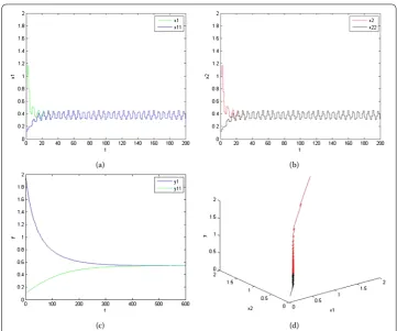
By calculation, these parameters of (6.2) meet the conditions of Theorem 3.1 and Corol-lary 5.1. Using MATLAB, by simulation, time series diagrams of (6.2) are shown in Fig-ure 2. FigFig-ure 2 shows that (6.2) is persistent and has a unique positive almost periodic solution which is globally attractive.
7 Conclusion
We construct a multispecies predator-prey model with mutual interference and time delays in this article. We obtain the conditions of permanence, global attractivity and uniqueness of positive almost periodic solutions of the system by using the Ascoli the-orem, Lebesgue dominated convergence thethe-orem, Lyapunov functions and comparison theorem. Finally, simulation results indicate the correctness of the theoretical results and demonstrate the complex dynamical behaviors of the system.
(a) (b)
(c) (d)
Figure 2 (a),(b)Time series diagrams with two initial values of preyxi(i= 1, 2), respectively.(c)The time
series diagram with two initial values of predatory.(d)Three-dimensional periodic diagram.
Acknowledgements
This paper is supported by the Natural Science Foundation of Guangxi (2016GXNSFAA380194), National Natural Science Foundation of China (11161015).
Competing interests
The authors declare that they have no competing interests.
Authors’ contributions
All authors contributed equally in this article. They read and approved the final manuscript.
Authors’ information
QL is now studying for the M.S. degree at Guilin University of Technology, Guilin, China. His research interest is the study of dynamical behaviors and simulation analysis of periodic impulsive differential equations. YS received Ph.D. degree in mathematics from Central South University, Changsha, China. He is a professor of School of Science, Guilin University of Technology, Guilin, China. His research interests are differential equations and dynamical systems. He is mainly engaged in qualitative studies of complex dynamical systems. SZ, ZW and HC are now studying for the M.S. degree at Guilin University of Technology, Guilin, China. Their research interests are stability analysis and numerical simulation of impulsive systems.
Publisher’s Note
Springer Nature remains neutral with regard to jurisdictional claims in published maps and institutional affiliations.
Received: 5 July 2017 Accepted: 8 December 2017
References
1. Holling, CS: The functional response of predator to prey density and its role in mimicry and population regulation. Mem. Entomol. Soc. Can.97(S45), 5-60 (1965)
2. Pei, Y, Chen, L, Zhang, Q, Li, C: Extinction and permanence of one-prey multi-predators of Holling type II function response system with impulsive biological control. J. Theor. Biol.235(4), 495-503 (2005)
3. Hassel, MP: Density dependence in single-species population. J. Anim. Ecol.44(1), 283-295 (1975)
5. Lin, X, Chen, F: Almost periodic solution for a Volterra model with mutual interference and Beddington-DeAngelis functional response. Appl. Math. Comput.214(2), 548-556 (2009)
6. Wang, K: Permanence and global asymptotical stability of a predator-prey model with mutual interference. Nonlinear Anal., Real World Appl.12(2), 1062-1071 (2011)
7. Lv, Y, Du, Z: Existence and global attractivity of a positive periodic solution to a Lotka-Volterra model with mutual interference and Holling III type functional response. Nonlinear Anal., Real World Appl.12(6), 3654-3664 (2011) 8. Zeng, G, Wang, F, Nieto, JJ: Complexity of a delayed predator-prey model with impulsive harvest and Holling type II
functional response. Adv. Complex Syst.11(1), 77-97 (2008)
9. Wang, K, Zhu, Y: Permanence and global asymptotic stability of a delayed predator-prey model with Hassell-Varley type functional response. Bull. Iran. Math. Soc.37(3), 197-215 (2011)
10. Du, Z, Lv, Y: Permanence and almost periodic solution of a Lotka-Volterra model with mutual interference and time delays. Appl. Math. Model.37(3), 1054-1068 (2013)
11. Shao, Y, Dai, B, Luo, Z: The dynamics of an impulsive one-prey multi-predators system with delay and Holling-type II functional response. Appl. Math. Comput.217(6), 2414-2424 (2010)
12. Bahaa, GM: Fractional optimal control problem for differential system with delay argument. Adv. Differ. Equ. (2017). https://doi.org/10.1186/s13662-017-1121-6
13. Wang, B, Cheng, J, Al-Barakati, A, Fardoun, HM: A mismatched membership function approach to sampled-data stabilization for T-S fuzzy systems with time-varying delayed signals. Signal Process.140, 161-170 (2017) 14. Cheng, J, Park, JH, Zhang, L, Zhu, Y: An asynchronous operation approach to event-triggered control for fuzzy
Markovian jump systems with general switching policies. IEEE Trans. Fuzzy Syst. (2016). https://doi.org/10.1109/TFUZZ.2016.2633325
15. Meng, X, Zhao, S, Zhang, W: Adaptive dynamics analysis of a predator-prey model with selective disturbance. Appl. Math. Comput.266, 946-958 (2015)
16. Aghajanzadeh, O, Sharif, M, Tashakori, S, Zohoor, H: Nonlinear adaptive control method for treatment of uncertain hepatitis B virus infection. Biomed. Signal Process. Control38, 174-181 (2017)
17. Rui, J, Liu, B: Almost-periodic solutions of an almost-periodically forced wave equation. J. Math. Anal. Appl.451(2), 629-658 (2017)
18. Meng, X, Chen, L: Almost periodic solution of non-autonomous Lotka-Volterra predator-prey dispersal system with delays. J. Theor. Biol.243(4), 562-574 (2006)
19. Chen, X: Almost periodic solutions of nonlinear delay population equation with feedback control. Nonlinear Anal., Real World Appl.8(1), 62-72 (2007)
20. Zhou, Z: Global attractivity and periodic solution of a discrete multispecies cooperation and competition predator-prey system. Discrete Dyn. Nat. Soc.2011, Article ID 835321 (2011)
21. Qiao, Y, Zhou, Z: Existence of positive solutions of singular fractional differential equations with infinite-point boundary conditions. Adv. Differ. Equ. (2017). https://doi.org/10.1186/s13662-016-1042-9
22. Miao, Z, Chen, F, Liu, J, Pu, L: Dynamic behaviors of a discrete Lotka-Volterra competitive system with the effect of toxic substances and feedback controls. Adv. Differ. Equ. (2017). https://doi.org/10.1186/s13662-017-1130-5 23. Chen, F: Almost periodic solution of the non-autonomous two-species competitive model with stage structure. Appl.
Math. Comput.181(1), 685-693 (2006)
24. Fink, AM: Almost Periodic Differential Equations. Springer, Berlin (1974)
25. Qi, W, Dai, B: Almost periodic solution forn-species Lotka-Volterra competitive system with delay and feedback controls. Appl. Math. Comput.200(1), 133-146 (2008)
26. Gopalsamy, K: Stability and Oscillations in Delay Differential Equations of Population Dynamics. Springer, Berlin (1992) 27. Zeng, G, Chen, L, Sun, L, Liu, Y: Permanence and the existence of the periodic solution of the non-autonomous
two-species competitive model with stage structure. Adv. Complex Syst. (2004). https://doi.org/10.1142/S0219525904000238
28. Shen, C: Permanence and global attractivity of the food-chain system with Holling IV type functional response. Appl. Math. Comput.194(1), 179-185 (2007)