A new key predistribution scheme for general and grid group deployment of wireless sensor networks

R E S E A R C H

Open Access

A new key predistribution scheme for general

and grid-group deployment of wireless sensor

networks

Samiran Bag

and Bimal Roy

Abstract

Key predistribution for wireless sensor networks has been a challenging field of research because stringent resource constraints make the key predistribution schemes difficult to implement. Despite this, key predistribution scheme is regarded as the best option for key management in wireless sensor networks. Here, the authors have proposed a new key predistribution scheme. This scheme exhibits better performance than existing schemes of its kind. Moreover, our scheme ensures constant time of key establishment between two nodes. We provide some bounds on the resiliency of this scheme.

Next, we use this new key predistribution scheme in a grid-group deployment of sensor nodes. The entire deployment zone is broken into square regions. The sensor nodes falling within a single square region can communicate directly. Sensor nodes belonging to different square regions can communicate by means of special nodes deployed in each of the square region. We measure the resiliency in terms of fraction of links disconnected as well as fraction of nodes and regions disconnected. We show that our key predistribution scheme when applied to grid-group deployment performs better than standard models in existence.

1 Introduction

Key predistribution in wireless sensor networks has attracted attention of researchers for a decade. Key predistribution schemes are classified into two groups viz. probabilistic key predistribution and deterministic key predistribution. In probabilistic key predistribution scheme, as the name implies, the keys are randomly drawn from a large pool of keys and are placed into the individual sensor nodes. This scheme does not ensure full con-nectivity between nodes. However, due to this scheme’s randomness, it does ensure resiliency against selective node capture attack. Some probabilistic schemes can be found in [1-3]. The main disadvantage of probabilistic key predistribution schemes are that they do not ensure full connectivity between each and every pair of nodes. On the other hand, in deterministic key predistribution scheme, a deterministic method is employed to load the keys into the sensor nodes. This scheme may or may not offer full connectivity between every pair of nodes of the Wireless

*Correspondence: [email protected]

Applied Statistics Unit, Indian Statistical Institute, 203 B T Road, Kolkata, WB 700108, India

Sensor Network (WSN). Several deterministic key pre-distribution schemes have been proposed by researchers. Blom [4] proposed a scheme for key for pairwise key establishment in a group of users. This scheme, though primarily not intended for WSNs, was later used for key establishment in WSN. A symmetric polynomial-based scheme was proposed by Blundo et al. in [5]. Key predis-tribution schemes based on combinatorial design can be found in [6-12].

Combinatorial designs have been extensively used in deterministic key management. Mitchel and Piper [13] first used this in key distribution. In combinatorial design-based key distribution, a set system is used. The elements of the set system are regarded as the keys. A block is regarded as the key ring of a node. Çamptepe and Yener [6,7] were first to use combinatorial designs for key predis-tribution in sensor networks. They used projective geom-etry and generalized quadrangles. Lee and Stinson [8,9] used transversal designs for key distribution. Chakrabarti et al. [11] proposed a hybrid key predistribution scheme by randomly merging the blocks of the transversal design proposed by Lee and Stinson. Their merging technique

enhances the resiliency of the key predistribution scheme of Lee and Stinson. Three designs were used by Dong et al. [14]. They also proposed a class of key predistribu-tion scheme based on orthogonal array [15]. Blackburn et al. [16] proposed Costas arrays and distinct difference configuration. Product construction was used by [17]. The scheme is based on the product of key distribution scheme and set systems. They deduce the conditions of the set systems that provide optimum connectivity and resiliency of the network. Ruj and Roy proposed several schemes using partially balanced design, transversal design, and Reed-Solomon codes [10,18,19].

Key predistribution in wireless sensor networks using deployment knowledge was first studied by Liu and Ning [3]. They proposed two predistribution schemes both of which took advantage of the deployment knowledge of sensor nodes. The first scheme called the closest pair-wise scheme was a modification of the pairpair-wise key pre-distribution scheme. The second prepre-distribution scheme uses the polynomial-based key predistribution scheme of Blundo et al. [5].

Several research works followed, e.g., [18,20-27]. In Du et al. scheme [20,21], the sensors are deployed in groups at a single point of deployment. The probability density function of the ultimate position of all sensors in a group are the same. They used multiple space Blom scheme [4] for key predistribution.

Yu and Guan [28,29] studied key predistribution schemes using deployment knowledge and compared the effect of deployment on triangular, hexagonal, and square grids. Huang et al. [24,25] proposed a grid-group-based key predistribution scheme. These schemes are perfectly secure to selective and random node capture attack. Here, the deployment area is divided into smaller rectangular zones of the same size. Every rectangular area contains equal number of sensors deployed uniformly in that zone. The keys in the sensors are deployed following multi-ple space Blom scheme similar to Du et al. scheme [20]. Each sensor node chooses keys from two key spaces such that no more than c sensors are chosen from the same key space, thus eliminating the possibility of node capture attacks. In [23], Zhou et al. discussed a key predistribution scheme where sensor nodes are mobile. There are static sensor which are deployed in groups. There are mobile collectors which are used to collect and aggregate sen-sor data and forward to the base station. The mobility of collectors enhance the data consistency.

Ruj and Roy [18] proposed a key predistribution for grid-group-based deployment. In this scheme, the deploy-ment area is divided into smaller square regions. There are n2such smaller regions. There are two types of nodes viz. common nodes and agents. Their scheme offers full con-nectivity between the set of agents of the regions within the communication range.

Bag proposed a key predistribution scheme using the deployment knowledge in [30]. Here, the author con-sidered a three-dimensional deployment zone where the sensor nodes are deployed not only along the length and breadth of the deployment zone but also along the height of the deployment zone.

In this paper, we propose a key predistribution scheme for homogeneous wireless sensor networks using the scheme of Blom [4] as well as symmetric balanced incom-plete block design (SBIBD). The main advantage of using this scheme for key predistribution is that for this scheme, the adversary needs to capture large number of nodes in order to compromise all the keys in an uncompromised node. In other words, in order to disconnect an uncap-tured node from all other nodes, the adversary needs to capture many more nodes than the other standard schemes.

Then, we use this new key predistribution scheme in a grid-group deployment of sensor nodes. A grid-group deployment refers to such a deployment where the entire deployment zone is broken into smaller two-dimensional square regions giving rise to ann×ngrid-group struc-ture. Equal number of sensor nodes are deployed in each of the smaller square regions of the deployment zone. Sensor nodes deployed inside one smaller square region forms a group. Sensor nodes within the same group com-municate more frequently than a pair of nodes falling in two different groups. This is driven by the fact that sen-sor nodes in proximity to each other communicate more frequently than distant nodes. Sensor nodes deployed in this fashion grid form a heterogeneous network. This type of deployment scheme is applied in battlefields where sensors belonging to a compromised zone need to be completely disconnected from the rest of the network. Because if an adversary compromises an area, all the sen-sor nodes deployed in that area are considered to be captured.

Our general key predistribution scheme offers better resiliency than the schemes in [4,6,7]. For example, in key predistribution scheme by Blom [4], the adversary can compromise all the keys of the entire WSN merely by cap-turingcnodes, wherec is the security parameter of the design. However, in our scheme, the adversary can only compromise few links by capturingcnodes. Our scheme also offers better resiliency than [6,7] in terms of the num-ber of links that get exposed when some nodes are com-promised. In both key predistribution schemes based on symmetric BIBD and generalized quadrangles in [6,7], the attacker can compromise many key links between pairs of uncaptured nodes by capturing a single node. However, in our scheme, the attacker needs to capture multiple nodes for compromising the key links between some pairs of nodes. We have compared our scheme with [18] and other similar schemes on the basis of fraction of links that gets exposed when some nodes get captured by the adversary. This is a well-known measure of the resiliency of a key predistribution scheme. Our scheme is shown to exhibit the best performance as far as the resiliency is concerned. The scheme of Ruj and Roy in [18] uses three times the number of supernodes we use in our scheme for full con-nectivity. Our scheme offers better resiliency using less number of supernodes.

2 Preliminaries

Here, we discuss some mathematical structures that we have used in our key predistribution scheme. Table 1 provides the meaning of different notations used in this section and in the next section.

2.1 Combinatorial design

A design [31] is a two tuple(X,A) where X is a set of varieties, andAis a set of subsets ofX:

A= {x:x⊆X}

Table 1 Table of notations

Notations

X The set of varieties of the design A The set of blocks of the design x1,. . .,xv The varieties ofX

B1,. . .,Bb Blocks ofA

GF(q) The finite field ofqelements

α The primitive element ofGF(q)

G Ac×rmatrix as defined below

t The total number of nodes in deployment

p A prime power wheret≤p2+p+1 N The set of nodes in deployment

f One to one mapN→A

Di c×csymmetric matrices overGF(q)fori=1, 2,. . .,v

A(v,b,r,k,λ)-BIBD is a design satisfying these proper-ties:

1. |X| =v. 2. |A| =b. 3. ∀B∈A,|B| =k.

4. ∀x∈X,|{B:B∈A,x∈B}| =r.

5. ∀x,y∈X,x=y,|{B:B∈A, x,y∈B}| =λ.

A(v,b,r,k,λ)-BIBD, wherev = b is called a symmetric BIBD or SBIBD.

It can be shown that in a symmetric BIBD,k=r[31]. A(n2+n+1,n+1, 1)-BIBD withn≥2 is called a pro-jective plane of ordern. It can be proven (Theorem 2.10, [31]) that for every prime powerq≥2, there exists a sym-metric(q2+q+1,q+1, 1)-BIBD i.e., a projective plane of orderq.

2.1.1 Construction of SBIBD

Çamptepe and Yener used mutually orthogonal Latin squares in constructing the key predistribution scheme of [6]. Another construction of the same scheme can be found in [32]. LetV3(q)be the set of a three-dimensional vector space over a finite fieldFqofqelements. A

projec-tive geometryPG(2,q)over a finite fieldFqis defined like

the following:

• The points are given by the one-dimensional subspaces ofV3(q).

• The lines are given by the two-dimensional subspaces ofV3(q).

• A point belongs to a line if the corresponding one-dimensional subspace of the point is contained in the two-dimensional subspace corresponding to the line.

• Two lines are incident to each other iff the intersection of the corresponding two-dimensional subspaces of them is a nonempty one-dimensional subspace.

It can be shown that there are(q3−1)/(q−1)orq2+q+1 number of distinct subspaces of dimension one ofV3(q) [32]. Similarly, the number of distinct subspaces of dimen-sion two ofV3(q)is alsoq2+q+1. Each two-dimensional subspace contains q + 1 distinct one-dimensional sub-spaces. The intersection of two-dimensional subspaces is a one-dimensional subspace ofV3(q). So, the number of points and lines inPG(2,q)isq2+q+1. Every line contains q+1 number of points. So, taking points as varieties and lines as blockPG(2,q)is a symmetric(q2+q+1,q+1, 1) BIBD.

Similarly, the points of PG(2,q) are one-dimensional subspaces ofV3(q). So, every variety of(q2+q+1,q+ 1, 1)SBIBD can be represented by the basis of the one-dimensional subspace it belongs to.

LetL1= {(1,s,t):s,t∈GF(q)}

L2= {(0, 1,s):s∈GF(q)} L3= {(0, 0, 1)}

Let,S=L1∪L2∪L3.

|S| =q2+q+1.

It can be shown that each element ofS is a basis of a distinct one-dimensional subspace ofV3(q). Throughout this article, we shall represent theq2+q+1 number of varieties of the(q2+q+1,q+1, 1)SBIBD by the elements ofS.

2.1.2 Shared variety discovery of(q2+q+1,q+1, 1)SBIBD Any two blocks of a symmetric(q2_{+q+1,q+1, 1)BIBD do} share one and unique variety. Given a(q2+q+1,q+1, 1) SBIBD, Algorithm 1 finds the common variety of two blocks of the design. This algorithm uses the basis of the nullspace ofA.x = 0. This basis can be computed using Gauss-Jordan elimination method [33,34] in a constant time. Therefore, the runtime of Algorithm 1 isO(1).

Algorithm 1Computing the shared variety between two

blocks of(q2+q+1,q+1, 1)SBIBD.

Require: Basis of block 1{(a1,b1,c1),(a2,b2,c2)}. Basis of block 2{(a₁,b₁,c₁),(a₂,b₂,c₂)}.

Ensure: Find the identifier of the shared variety of the two blocks.

A= ⎡

⎣a1 a2 −a

1 −a2 b1 b2 −b1 −b2 c1 c2 −c1 −c2 ⎤ ⎦,x=

⎡ ⎢ ⎢ ⎣

x1 x2 x3 x4 ⎤ ⎥ ⎥ ⎦

Find the basis of the nullspaceA.x=0. Let this basis be given by(β1,β2,β3,β4). a=a1β1+a2β2

b=b1β1+b2β2 c=c1β1+c2β2 ifa=0then

The identifier of the common variety is (1,a−1b,a−1c).

else

ifb=0then

The identifier of the common variety is(0, 1,b−1c). else

The identifier of the common variety is(0, 0, 1). end if

end if

2.2 Key predistribution using combinatorial design Once we have a(v,b,r,k,λ)-design(X,A), we can map it to a key predistribution scheme in the following way:

LetKbe a set ofvkeys.

N be a set ofb nodes in the WSN.

LetA= {B1,B2,. . .,Bb}be the blocks of the design.

Letf :K→Xbe a map andg:N →Abe another map.

For eachBi∈A,i=1, 2,. . .,band

∀aj∈X,j=1, 2,. . .,vifaj∈Biand bothf−1(aj)

andg−1_(B

i)exist, load keyf(aj)into nodeg(Bi).

In plain language, what we do here is to use varieties as keys and blocks as node. A node corresponding to a block contains all the keys corresponding to the varieties that the particular block contains. Two nodes will have a common key if and only if the corresponding blocks do share at least one common variety. Again, the number of keys in a node will be equal to the number of varieties in a block that corresponds to the node.

2.3 Blom’s scheme

Blom [4] proposed a scheme for key predistribution where the members of a group can establish pairwise keys. Let Nbe the size of the network. The distribution server first chooses ac×N matrixGover a finite fieldGF(q). The matrixGis considered to be a public information. Now, the distribution server constructs ac×csymmetric matrix DoverGF(q). This matrix is a private information of the system. Now, the server computes the c×N matrixA, where A = (DG)T, T being the transposition operator. Now,AG = (DG)TG = GTDTG= GTDG= GTAT = (AG)T.

Thus,AGis a symmetric matrix. LetK =AG, we know that Kij = Kji, whereKij is the element inK located in

theith row andjth column.Kij(orKji) is the pairwise key

between node Ui and node Uj. To carry out the above

computation, nodes Ui and Uj should be able to

com-puteKij andKji, respectively. This can be easily achieved

using the following key predistribution scheme, forw = 1, 2,. . .,N,

• Store thewth row of matrixA in nodeUw. • Store thewth column of matrixG in nodeUw.

Now, if two nodes (sayUx andUy ) want to

communi-cate, they need to establish a common key. NodeUxhas

rowxofAand columnxofG. NodeUyhas rowyofAand

columnyofG. Now , they can establish a pairwise key this way:

• NodeUxandUyexchange columnx and column y of

matrixG, respectively.

The matrix G is a public information. Therefore, the rows ofGcould be sent without encryption. SinceKis a symmetric matrix,Kxy = Kyx. Hence,Kxycan be used as

the common key between the two nodes.

2.3.1 c-secure property

It has been proved that the above scheme isc-secure [4], i.e., if anyc+1 columns ofGare linearly independent; then, no member other thanUxandUycan computeKxy

orKyxif no more thancmembers are compromised.

2.3.2 A construction for matrix G

We note that anyc+1 columns ofG[35] must be linearly independent in order to achieve thec-secure property. Let αbe a primitive element of a finite fieldGF(q)whereqis a prime power.

A feasible G can be designed as follows [36]:

G= erty of primitive elements). Since G is a Vandermonde matrix, it can be shown that anyc+1 columns ofGare lin-early independent whenα,α2,α3,. . .,αN are all distinct. In practice,Gcan be generated by the primitive elementα ofGF(q). Therefore, thewth column ofGis stored at node Uw; it is only required to store the seedαw, and any node

can regenerate the column given the seed.

2.4 Threat model

Wireless sensor nodes are deployed in unattended envi-ronment often in an area under the control of adversaries. Thus, the sensor nodes that gather and communicate sen-sitive information are vulnerable to attacks. An active adversary can physically capture a number of nodes, and it can get to know the stored keys into them. These keys can thereafter be used by the adversary to decrypt messages communicated across sensor nodes. We shall discuss two types of attacks to our proposed scheme.

2.4.1 Random node capture

In this type of attack, the adversary randomly captures nodes from the deployment zone and exposes the keys loaded into them.

2.4.2 Selective node capture

This attack was first introduced in [37]. An active attacker is in attempt to obtain a setTof keys. For achieving this, the attacker is compromising sensor nodes. It has already obtained a set of keysSthis way, whereS ⊂ T. For each

node s in the WSN, the random variable G(s) is equal to the number of keys belonging to T \S; the attacker gains by compromisingsnodes. At each step of the attack sequence, the next sensor to be tampered with is sensor s, wheresmaximizesE[G(s)|I(s)], the expectation of the key information gainG(s)given the informationI(s)that the attacker knows on sensors’s key ring.

3 Proposed scheme

3.1 Key predistribution in the group

Here, our aim is to design a key predistribution scheme for a sensor network consistingNnodes whereN ≤p2+p+1 wherepis a prime number.

We use the scheme in [6,7] by Çamtepe and Yener and Blom’s scheme [4]. This scheme is based on symmetric design (Section 2) . They used a symmetric (p2 +p+ 1,p+1, 1)design to build a key predistribution scheme for WSN.

We shall be using a(p2+p+1,p+1, 1)-symmetric balanced incomplete block design (X,A). Here, X = {x1,x2,. . .,xv},v = p2 + p + 1. A = {B : B =

Definition 2.f is a one-to-one map from the set of nodes of the sensor network to the blocks of the symmetric(p2+ p+1,p+1, 1)design. In addition to that, we assume that f−1can be computed in constant time.

It can be noted that the nodes can be identified by the identifier of the blocks they correspond to. Therefore, one example of the functionf is the identity mapping ifN ⊆A.

value the integerc. Now, compute p2+p+ 1 symmet-Section 2.1 into a key predistribution scheme. LetN = {n1,n2,. . .,nt} be the set of nodes in the WSN. We

can design a key predistribution in these nodes using Algorithm 2 and takingv= b = p2+p+1,r = p+1. In Algorithm 2, we takev = p2+p+1 many different key spaces of the Blom scheme [4]. We compute onec×r public matrixGand a set ofvmanyc×csecret symmet-ric matrix Di,i ∈ {1, 2,. . .,v}. Thus, we can computev

manyAmatrices like this :Ai=(DiG˙)T. Hence, there are

vmany distinct key spaces of Blom scheme. Now, we can have a key distribution scheme by considering each of the vkey space as a variety of the(p2+p+1,p+1, 1)- SBIBD, where each block of the SBIBD corresponds to a node of the WSN. Since a block of a(p2+p+1,p+1, 1)- SBIBD containsp+1 many varieties, every node will have its key share from exactlyp+1 many key spaces.

Algorithm 2Algorithm for key predistribution in nodes. Require: A combinatorial design(X,A)where

X= {x1,x2,. . .,xv}, Ensure: A key predistribution in sensor nodes ofN.

for allxj∈X, 1≤j≤vdo

It is easy to see that one nodenhcontains one row from

each matrix of the set M_h whereM_h ⊂ {A1,A2,. . .,Av} In this designk=p+1. Therefore, the memory overhead isO(p)orO(√|N|).

3.1.3 Shared key discovery between two nodes

Two nodes wishing to communicate securely need to agree upon a secret key. In the scheme discussed in Section 3.1.1, any two nodes can surely compute a shared key. We provide an algorithm that takes all arguments of Algorithm 2 and finds a shared key between two nodes. In addition, the algorithm takes two nodes as input and finds a common key shared by both of them.

The most costly computation of Algorithm 3 is at step 3. This step reduces in finding all the blocks of a design that contains a particular variety. This can be found using a different construction of symmetric BIBD as discussed in Section 8.4 of [32].

Algorithm 3 Algorithm to compute common key

between nodeniannj.

Require: Combinatorial design(X,A)used in Algorithm 2 where

Ensure: Compute the common key between nodeni

andnj

1) Let,By=f(ni),Bz=f(nj)

2) Computexm∈X,m∈ {1, 2,. . .,v}such thatxm∈

By∩Bz

3) Findu=POS(By,xm)andw=POS(Bz,xm)

4) Computewth column of matrixGfrom (α,α2,. . .,αr).

5) Kni,nj =(uth row of matrixAm).(wth column of matrix G)

Time complexity of Algorithm 3 The first step reduces

belonging to two different blocks in the design used in Algorithm 2. Note that in a(p2+p+1,p+1, 1)-SBIBD, any two blocks will share a unique common variety. Com-puting such a variety in a (p2_{+p+1,p+1, 1)-SBIBD} is equivalent to computing a basis of the intersection of two-dimensional subspaces. This can be done in con-stant time using the Algorithm 1. The third step is a lookup of memory and is, too, of time complexity O(1) if the items are stored in an indexed table. In the fourth step, the wth column of matrix G is calculated which is given by (1,αw,(αw)2,(αw)3,. . .,(αw)c−1). Since the nodes storeαifor eachi=1, 2, 3,. . .,randcis a constant, so computing thewth column of matrixGrequiresO(1) computation. Finally, the fifth step can also be done in constant time since the vectors are of constant dimension. Therefore, the overall runtime of Algorithm 3 isO(1).

Note that node ni stores the value u = POS(By,xm)

in the Algorithm 3, and nodenjstores the value ofw =

POS(Bz,xm). However, for computing the shared key, both

the nodes need the values ofuandw. So, the two nodes must exchange the values of u and w which will incur an additional communication cost ofO(1). To avoid this, every node can store the values of POS(∗,∗) for other nodes. For example nodeni =f−1(By)needs to store the

values ofPOS(Be,xl) : 1 ≤ e ≤ v,e = y,xl = BeBy.

This will require a memory overhead ofO(N).

3.2 Proof of correctness of algorithms

Here, we establish the correctness of Algorithm 2 and Algorithm 3. It will be sufficient to show that after deploy-ment, a pair of distinct nodes ni and nj, 1 ≤ i,j ≤ v

will be able to compute their common keyKninj = Knjni using the shared key discovery method of Algorithm 3. According to Algorithm 3, both nodeniand nodenjwill

compute the blocks By = f(ni) and Bz = f(nj). Now,

they can find the common elementxm ∈ By

Bz : 1 ≤

m ≤ v using Algorithm 1. Now, nodeni will compute

u = POS(By,xm). Similarly, nodenj will calculatew =

POS(Bz,xm). Node ni andnj will exchange the valuesu

andv. Nodeniwill compute thewth column of matrixG

from(α,α2,. . .,αr)stored in it. Similarly, nodenjwill

cal-culate theuth column of matrixGfrom(α,α2,αr)stored in it. From Algorithm 1, we can see that nodeni andnj

have got theuth andwth row of matrixAm = (Dm.G)T.

Hence, nodenican computeKuw = (uth row of matrix

Am).(wth column of matrix G. Node nj will compute

Kwu = (wth row of matrixAm).(uth column of matrix

G in a similar way. Since Am.G is a symmetric matrix,

Kuw = Kwu = Kninj. Hence, the two nodes will end up computing the same key using Algorithm 3. Therefore, the Algorithm 2 and 3 are correct. It can be noted that any row of matrixAk, 1 ≤ k ≤ vis contained only in exactly one

node according to Algorithm 2. So, only nodenicontains

theuth row ofAmand only nodenjcontains thewth row

ofAm. Hence, no other node can compute the common

keyKninj.

4 Performance analysis of proposed scheme

In this section, we shall investigate the security aspects of the proposed scheme. As discussed in Section 1, sen-sor nodes are deployed in unattended environment often in area controlled by an adversary. So, an active adversary can compromise one or more sensor nodes of the deploy-ment zone. If the sensor nodes are not tamper proof, the adversary can extract sensitive information from the set of sensor nodes compromised by the adversary and can use those informations to overhear the conversation between active sensor nodes.

Lemma 3.For the proposed scheme, letSbe the set of compromised sensor nodes. Let, f(S)= {f(n):n∈S}. Two uncompromised nodes n1and n2will have an uncompro-mised link between them if and only if|{B:B∈f(S)&x∈ B}| ≤c−1, where x=B1∩B2and f(n1)=B1,f(n2)=B2.

Proof.Follows from the fact thatcis the security param-eter of the scheme in Section 2.3.

Let, x = xκ, where κ ∈ {1, 2,. . .,v}. Then by Algorithm 2 and 2.3, it can be said that if the matrixAκcan be compromised, then the common key between noden1 andn2can be computed. This can only be possible if and only if anycnumber of rows of the matrixAκare compro-mised. Letψ = {n:n∈N&xκ ∈f(n)}. Hence, the nodes inψ contain one distinct row ofAκ each. So, successful computation of the shared key is possible if and only if |S∩ψ| ≥ c. In other words, the common key between the two nodesn1andn2will remain active if and only if |{B:B∈f(S)&x∈B}| ≤c−1.

Proposition 4.Let the total number of nodes be N and the security parameter be c. If s number of nodes are compromised and s≥ c, the probability that two uncom-promised nodes will have an uncomuncom-promised link is given

by c−1

e=0(k−e2)(N−ks−e) (N−2

s ) .

Proof.Let C denote the event that the two nodes will share an uncompromised link. Let the two nodes be given by n1 andn2. Let, f(n1) = B1 andf(n2) = B2, where B1,B2 ∈ A. There must be a uniquexi ∈ X such that {xi} = B1∩B2. Again, let the set of compromised nodes beS, where |S| = s. The adversary cannot compute the shared key betweenn1andn2iff|{B:B∈f(S)&xi∈B}| ≤

c−1. In a symmetric(v,k,λ)design, there areknumber of blocks containing a particular variety. So, for any par-ticular varietyxi ∈ X,|{B: B∈ A&xi ∈ B}| =k. Again,

B1,B2∈ {B:B∈A&xi ∈B}. Therefore,|{B:B∈A&xi ∈

P(|{B:B∈f(S)&xi ∈B,n1,n2∈/S}| =e)= (

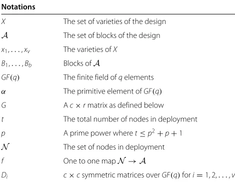
We provide the values of P(C) for different sets of parameters in Table 2. It can be seen that our scheme has high probability of existence of a live link between two uncaptured nodes even when large number of nodes are compromised. Here,pis the prime number of the sym-metric balanced incomplete block design that is used in the scheme.cis the security parameter of Blom’s scheme. sis the number of compromised nodes. Table 2 shows that this scheme has a high probability of existence of a key link between two nodes even when many nodes are compro-mised. Also, ifpincreases, the number of nodes increases and so does the probability of existence of a link between a pair of nodes.

4.1 Performance analysis in terms of known measures We shall analyze the performance of our scheme in terms of two well-known measures viz.E(s)andV(s). These are the standard measures used for evaluating the resiliency of any key predistribution scheme.

Definition 5.E(s)is defined to be the ratio of the num-ber of links exposed in the network when s numnum-ber of nodes are compromised to the number of links present in the network before s number of nodes were compromised.

Let, L be the total number of links in a network and l be the number of links exposed after s number of nodes are compromised.

then E(s)= _Ll

Here, we will consider only the resiliency of the subnet-work consisting of nodes.E(s)is the measure that shows

Table 2 Probability of existence of an active link between two uncompromised nodes in our scheme for different parameters

p c s Probability of existence of link

37 4 34 0.998651

Here,pis the prime number,sis the number of compromised nodes, andcis the security parameter of the scheme.

the performance of the scheme in terms of it’s resiliency against node captures. As defined above,E(s)is the mea-sure that shows the fraction of links that gets exposed whensnumber of nodes get compromised. So, the lesser the value ofE(s) is, the more resilient is the scheme to

0 if the adversary can compute the common key between nodeniand

njusing the information stored in

nodesnκ,κ ∈S

We take the attacker’s point of view who would try to expose more links through compromising as less num-ber of nodes as possible. In our design, a link can be exposed only if at leastc number of nodes are compro-mised that contain one row of matrixAh, each for some

h ∈ {1, 2,. . .,v}. Ifcnumber of rows are compromised, then the attacker would be able to reconstruct the matrix Ah. SinceAis a(p+1)×c, the attacker would be able to

would be able to reconstruct matrix Ai and hence, the

links between nodes n0,n1,. . .,np will get exposed. So,

the total number of exposed links will be p+₂1. Let the set of nodes compromised by the advisor for obtainingAi

The attacker can do this through compromising another matrixAj,j = h,j ∈ {1, 2,. . .,v}. This time, the attacker

needs to compromisec−1 nodes. First, an attacker selects a j = h such that a node in S does contain a row Aj.

Choosing such ajwill ensure that the attacker will have to compromisec−1 more nodes. It can be proved that for anyj = h, there is at most one node inS that con-tains a row of matrixAj. So, the attacker would require

to compromisec−1 additional nodes for exposingp+₂1 links. This way, it can be proved that the attacker would require to compromisec−2 nodes for exposing the next set of p+₂1 number of links and so on. This way, the attacker can compromisecp+₂1number of links by cap-turingc+(c−1) +(c− 2)+ . . .+1 nodes or c(c+₂1) nodes.

Hence, fors≤ c(c₂+1),E(s)≤cp+₂1/p2+₂p+1or,E(s)≤ c

p2_+p+1.

Theorem 6 gives an upper bound of the extent of dam-age that occurs to the subnetwork consisting of nodes. Sincep2+p+1 >>c, soE(s)is very close to zero or, in other words, the number of links that get exposed is small when less thanc(c+₂1) number of nodes are captured.

Lemma 7.If a set ofSsensor nodes get captured, then a node ni ∈/ Swill get disconnected from the rest of the

network if and only if∀x∈f(ni),|{B:B∈f(S),x∈B}| ≥

c.

Proof.The proof follows from Lemma 3 and thec secu-rity property.

Definition 8.V(s)is the fraction of nodes that get dis-connected from the rest of the networks. Let m be the

number of uncompromised nodes that get disconnected from the rest of the network of size N when s nodes are compromised, then V(s)= _N−m_s−m.

Theorem 9.V(s)=0,∀s< (p+1)c.

Proof.Let the attacker wants to disconnect a particu-lar nodeni,i ∈ {1, 2,. . .,v}from the rest of the network.

Let,Sbe the minimal set of nodes that the attacker needs to capture for disconnecting the first (uncompromised) node from the rest of the network. LetBj = f(ni),j ∈ {1, 2,. . .,v}. Hence,Bj ∈ X. Let,{x1,x2,. . .,xp+1} = Bj.

Let∀k∈ {1, 2,. . .,p+1},Ck = {B:B∈f(S)&xk ∈B}. It

can be seen thatf(S)= ∪p_k+₌₁1Ck.

We claim thatCk ∩C_k = φ,k =k, 1 ≤ k,k ≤p+1.

If not, then suppose there exists a blockBm ∈ Ck ∩C_k.

Hence,xk,x_k ∈Bm. So,|Bm∩Bj| ≥2. This is not possible

since the design we used is a symmetric(p2+p+1,p+1, 1) design. So our assumption is wrong.

From the c-security property, we can say that |Ck| =

c∀k ∈ {1, 2,. . .,p+1}. Hence,|f(S)| = |S| = (p+1)c. Hence the result.

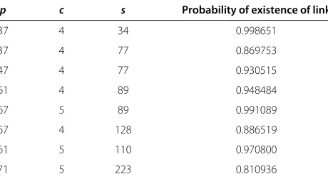
The performance of our scheme in terms ofV(s)for cer-tain value of parameters is shown in Figure 1. It can be seen that the value ofV(s)in Figure 1 is in agreement with the result stated in Theorem 9.

4.2 Comparative study of the scheme

Here, we compare the resiliency of our proposed scheme with other existing schemes. Some well-known standard schemes are the basic scheme of Eschenauer and Gligor [1], Lee and Stinson’s quadratic and linear scheme based on transversal design in [8,9,38], Çamptepe and Yener’s

scheme in [7], the scheme of Chakrabarti et al. [11], and partially balanced incomplete block design based scheme by Ruj and Roy in [10].

The scheme of Eschenauer and Gligor in [1] is a prob-abilistic key predistribution scheme. This scheme uses a pool of keys. Keys are drawn randomly from the key pool with replacement and are placed in the sensor nodes. All nodes are loaded with same number of keys. This scheme does not ensure the existence of a common key between a pair of nodes. This scheme is known as the basic scheme.

Lee and Stinson [8,38] used transversal design in key predistribution. They proposed two types of transversal design viz. linear and quadratic. In these schemes, a pair of nodes can have zero or one key in common. They used the following construction of a transversal designTD(k,r) [8].

1. X= {(x,y): 0≤x<k, 0≤y<r}. 2. ∀i,Gi= {(i,y): 0≤y<r}.

3. A= {Ai,j: 0≤i<r&0≤j<r}.

They defined blockAi,jbyAi,j=(x,xi+j modr): 0≤

x< k, 0≤i,j< r. Similarly for a quadratic scheme, they defined a blockAi,j,k by Ai,j,k =

x,xi2+xj+k modr: 0≤x<k, 0≤i,j<r.

Each block is assigned to a node. So, the linear Lee-Stinson’s scheme supports r2 nodes, and the quadratic scheme supports as many asp3nodes.

Çamtepe and Yener used symmetric balanced incom-plete block design in [7]. A SBIBD is a(p2+p+1,p+1, 1) design where p is a prime number. They used projec-tive geometry for constructing the SBIBD. This scheme ensures full connectivity between nodes. Each node in this

scheme containsp+1 keys, and every key is contained in p+1 nodes.

Chakrabarti et al. [11] proposed a hybrid key predis-tribution scheme by merging the blocks in combinatorial designs. They considered the blocks constructed from the transversal design proposed by Lee and Stinson and randomly selected them and merged them to form the sensor nodes. Though this scheme increases the number of the keys per node, it improves the resiliency of the net-work. The probability that two nodes share a common key is also high. Thus, it has a better connectivity.

Ruj and Roy proposed two schemes for key predistri-bution in [10]. They used partially balanced incomplete block design. In the first scheme, the number of nodes as well as the number of keys are equal ton(n−1)/2 for some positive integern. The number of keys in a node is equal to 2(n−2). The number of nodes containing the same key is also 2(n−2). They presented another design that aug-ments the size of the network, keeping the same number of keys in each node. The keys in the key pool also remain the same. They showed that network size can be increased in steps, keeping the same number of keys per node. How-ever, to ensure that any pair of nodes can communicate directly, we cannot go on adding nodes in this scheme.

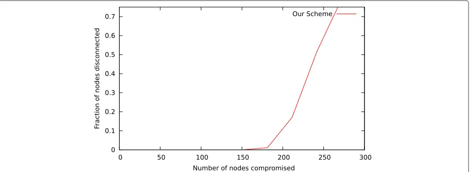
We have defined E(s) in Section 4.1. E(s) is the best measure of resiliency of any key predistribution scheme. A key predistribution scheme for which the value ofE(s) is lower offers better resiliency against node capture. So, a key predistribution scheme having low value of E(s) for different values of captured nodes can withstand key compromise. Figure 2 shows a comparison between our scheme with these schemes in terms ofE(s). We measured the resiliency of the key predistribution schemes by means

of simulation. The parameters of different key predistri-bution schemes and the number of nodes in the WSN are given in Table 3. We have chosen nearly equal sizes of networks for different schemes in consideration. The other parameters are chosen depending upon the network size and the system models so that the key predistribu-tion schemes exhibit optimal performance.Nis the total number of nodes in the network, andkis the number of keys per node. The value ofk depends upon the other parameters of the network which in turn depend upon the network size. The last column of Table 3 shows whether the key predistribution scheme ensures full connectivity among the nodes or not. We used C program to evalu-ate the values ofE(s) for different values of sfor all the schemes mentioned above. We compiled the source using GNU C compiler GCC 4.5.4. We considered random node capture by the adversary. In Figure 2, the line correspond-ing to the performance of our scheme almost touches the x-axis throughout the range. Hence, it can be inferred that less number of links get exposed in our scheme as com-pared to other schemes when same number of nodes are captured by the adversary. In other words, our scheme offers better performance than all the other schemes in terms ofE(s). The reason why our scheme excels in per-formance can be inferred from Lemma 3. Lemma 3 says that in order to compromise the links between any two nodes, the adversary is required to compromise at least c(cis the security parameter) nodes having information from the same key space as the two nodes. However, in other schemes, the same thing can be done by capturing a single node. So, even if the number of captured nodes is high enough, the value ofE(s) can be very low in our scheme. This fact is corroborated by the performance of our scheme as shown in Figure 2.

5 New grid-group deployment-based design

We shall use our proposed key predistribution scheme in developing a key predistribution scheme for

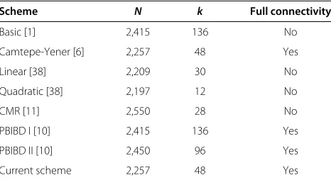
grid-Table 3 Schemes with parameters that we choose for our comparisons and connectivity

Scheme N k Full connectivity

Basic [1] 2,415 136 No

Camtepe-Yener [6] 2,257 48 Yes

Linear [38] 2,209 30 No

Quadratic [38] 2,197 12 No

CMR [11] 2,550 28 No

PBIBD I [10] 2,415 136 Yes

PBIBD II [10] 2,450 96 Yes

Current scheme 2,257 48 Yes

Nis the total number of nodes in the network, andkis the number of keys in a node.

group deployment. As mentioned earlier in Section 1, a grid-group deployment refers to such deployment where the entire network is broken into smaller regions called groups. The sensor nodes belonging to one group could be deemed as a mini-WSN where the sensors of a certain group communicates among themselves more frequently than with sensors of different groups. We propose a key predistribution scheme for a WSN where the network is divided into aN×Nsquare grid. Each group in this group has got identical number of sensors.

5.1 The scheme

Letpbe a prime number. LetN ≤p2+p+1 be the number of sensors in each group. The groups are denoted by the two tuple(i,j), 0≤i,j≤N. We shall denote the nodes of any group(i,j)asnl_ij, 0≤l≤t−1. We designate one node from each group as a supernode. This supernode has got more amount of resources than ordinary nodes in terms of memory, computational power, battery power, etc. This special node will be used for intergroup communication. The supernode of group(i,j)is denoted bySi,j. It can be

noted that a supernodeSi,jof any group(i,j)does belong

to the set{nl_ij : 0≤l≤t−1}. If a nodenα_i,jof group(i,j)

wants to communicate with nodenβ_i,jof group(i,j), then the following steps are taken:

• Nodenα_i,jgenerates a random keyK.

• Nodenα_i,jsendKto the supernodeSij. • SijpassesKtoSij.

• SijsendsKto nodenβi,j.

Now, the two nodes viznα_i,jandnβ_i,j can communicate using the keyK.

It can be noted that for accomplishing all the steps mentioned above, it is necessary to have:

1. Any two pair of nodesnα_i,jandnα_i,jbelonging to group

(i,j)must be able to communicate securely

∀α∈ {0, 1, 2,. . .,t−1}and0≤i,j≤p−1.

2. Any pair of supernodesSi,jandSi,j belonging to two

different groups(i,j)and(i,j)must be able to communicate securely where

0≤i,j,i,j≤p−1,(i,j)=(i,j).

hands of the adversary, the keys in sensor nodes in other groups remain unaffected. It should be kept in mind that a supernode belongs to the group corresponding to the square region they are deployed in. Hence, a supernode contains two types of keys, one that allows it to commu-nicate securely with other nodes in the same group they belong to and the other that allows it to communicate with other supernodes belonging to different groups. There-fore, the key predistribution in the whole network looks like the following :

1. Key predistribution for each of theN2groups is done by using the scheme of Section 3 using exclusive key spaces for all the groups.

2. A separate key predistribution using the same scheme of Section 3 is done for all the supernodes belonging to all the groups.

We assume that it is hard to capture a supernode until the entire square region where the supernode is located is compromised. We have assumed that the nodes within the same square region communicate more frequently than the two nodes each belonging to a separate square region. Hence, one supernode per group is sufficient to handle the burden of intergroup communication.

5.2 Resiliency of the network

When it comes to the resiliency of the key predistribution scheme in a grid-group deployment of the sensor network, there are three types of resiliency:

• Intragroup resiliency : resiliency within a certain group.

• Resiliency of the interlinks : resiliency in the set of supernodes.

• Overall resiliency : resiliency of the entire network.

Within a group, the nodes work as a single WSN. Hence, the resiliency of the key predistribution is same as in Section 4. In this section, we study the resiliency of the interlinks in our key predistribution scheme. Here, too, similar to Section 4, we shall be using the standard mea-sures for evaluating the resiliency of our scheme. The two measures we shall be using areE(s)andV(s).

Definition 10.E(s)is defined to be the fraction of inter-links between groups that get exposed when s number of supernodes are captured by the adversary. In other words, E(s)is the ratio of the interlinks present in the grid after s many supernodes are captured to the number of inter-links present in the network before s many supernodes are captured.

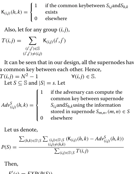
LetS= {(i,j): 0≤i,j≤N−1}

K(i,j)(h,k)= ⎧ ⎨ ⎩

1 if the common keybetweenSi,jandSh,k

exists 0 elsewhere

Also, let for any group(i,j),

T(i,j)= (i,j)∈S (i,j)=(i,j)

K(i,j)(i,j)

It can be seen that in our design, all the supernodes have a common key between each other. Hence,

T(i,j)=N2_{−1 ∀(i,j)∈S.} LetS⊆Sand|S| =s. Let

AdvS_(i,j)(h,k)= ⎧ ⎪ ⎪ ⎪ ⎪ ⎨ ⎪ ⎪ ⎪ ⎪ ⎩

1 if the adversary can compute the common key between supernode

Si,jandSh,kusing the information

stored in supernodeSm,n,(m,n)∈S

0 elsewhere

Let us denote,

P(S)=

(h,k)∈S\S (i,j)∈S\S (i,j)=(h,k)

(K(i,j)(h,k)−AdvS_(i,j)(h,k))

(i,j)∈S\ST(i,j)

Then,

E(s)=EXP(P(S)),

0 0.05 0.1 0.15 0.2 0.25 0.3 0.35 0.4 0.45

0 10 20 30 40 50 60 70 80 90

F

raction of links e

xposed

Number of nodes compromised

Our Scheme Scheme of Ruj Roy

Figure 3Graphical comparison of fraction of interlinks disconnected.This comparison is done with respect to the number of supernodes compromised for our scheme and the scheme in [18].

scheme, less number of links will get broken than the Ruj-Roy scheme when the same number of nodes are captured. So, in our scheme, more interregion links remain intact than the Ruj-Roy scheme when some supernodes are cap-tured. Thus, our scheme exhibits better performance than the Ruj-Roy scheme though it makes use of only one-third of the number of supernodes used in Ruj-Roy scheme. Our scheme reduces the cost incurred due to the deploy-ment of large number of supernodes and also enhances the resiliency of the network against node capture.

Definition 11.V(s) is the fraction of groups that are disconnected from the rest of the groups with respect to the total number of groups when s number of supernodes are captured. In other words V(s)is the ratio of the number of groups that do not have any link to other groups after the s number of supernodes are captured to the total number of active supernodes present in the network before s many supernodes are captured.

The result proved in Theorem 9 is also applicable for the interlinks between supernodes in different groups. Hence, for our scheme, individual groups do not get disconnected from the rest of the network unless a large number of supernodes get captured.

Table 4 Parameters used in comparison of the proposed scheme and the Ruj and Roy scheme in Figure 3

Parameters Ruj-Roy scheme Scheme of the

current study

Number of square regions 1,369 1,369

Security parameter - 4

Number of keys per node 13

-Total number of nodes 4,107 1,369

Figure 4 shows the comparative performance of our scheme, and the Ruj-Roy scheme where the comparison is done in terms ofV(s). The parameters of the graphi-cal plot of Figure 4 is shown in Table 5. As defined above, V(s) is the fraction of nodes that get entirely discon-nected from the rest of the network when s number of nodes get exposed. We used a 37×37 square grid in each case. The total number of supernodes in the entire net-work is 4, 107 in Ruj-Roy scheme and 1, 369 in our scheme. We have taken the security parameter of our scheme to be 4. The value ofpin our scheme is 37. The number of keys (k) in a supernode is 23 in Ruj-Roy scheme. We used C program to evaluate the values ofE(s)for different values ofsfor both schemes. We compiled the source using GNU C compiler GCC 4.5.4. Figure 4 shows that in our scheme, less number of nodes get detached from the network than the Ruj-Roy scheme in [18] when same number of nodes get captured by the adversary. Hence, our scheme is bet-ter than the Ruj-Roy scheme as it can keep more nodes connected to the network.

5.3 Overall resiliency

0

Figure 4Graphical comparison of fraction of nodes disconnected.This comparison is done with respect to the number of nodes compromised for our scheme and the scheme in [18].

supernodes remaining in the network. We are the first to propose this as a measure of overall resiliency in terms of fraction of links exposed in the entire network. In this measure, we separately compute the values of fraction of links exposed(E(sij)) in every region (i,j) : 0 ≤ i,j ≤

N − 1. We also measure the value of E(s) among the set of supernodes in the network. Then, we compute the weighted average of all these values ofE(s).

Here, we take into account the entire network consisting of all the nodes and supernodes in all the regions. Letsijbe

the number of nodes compromised in group(i,j)ands=

sg many supernodes are compromised. After sij many

nodes are compromised in region (i,j), the number of uncompromised nodes present in region(i,j)isN −sij.

Hence, the weight corresponding to any region (i,j) is _N−sij

2

which is equal to the number of pairs of uncom-promised nodes in region (i,j). Similarly, for the set of supernodes, the weight assigned isN2−sg

2

Table 5 Parameters used in comparison of the proposed scheme and the Ruj and Roy scheme in Figure 4

Parameters Ruj-Roy scheme Scheme of the

current study

Number of square regions 1,369 1,369

Security parameter - 5

Number of keys per node 23

-Total number of nodes 4,107 1,369

Hence, when the number of nodes captured from dif-ferent groups is fixed, the overall E(s) is the weighted average of the value ofE(sij)of all groups and the group of

all supernodes.

Lemma 12.When sij number of nodes are

compro-mised in group (i,j), 0 ≤ i,j ≤ N − 1 then E(s) < which includes one supernode. Ifsijnumber of nodes are

captured in group(i,j), the probability that the supernode will get captured is sij

p2_+p+1. In order to expose at least one link between two uncompromised supernodes, the adver-sary will have to compromise at leastcnodes containing informations from the same key space of our scheme. The probability of compromisingcmany supernodes contain-ing information from the same key space is very close to zero. Hence,Eg_(s

Corollary 13.When sij number of nodes are

compro-mised in group(i,j), 0≤i,j≤N−1then E(s) < _p2+c_p+1

with a high probability where s= N_i=−₀1 _jN₌−₀1sijand s is

not-so-large and for all(i,j): 0≤i,j<N,sij≤ 1₂c(c+1).

Proof.Follows directly fromLemma12 andTheorem6.

Corollary 13 gives an upper bound of the numeric value of fraction of links disconnected in the set of all uncom-promised nodes of the network.

Definition 14.V(s)is defined to be the weighted aver-age of the fractions of nodes disconnected from the rest of the network in a region (i,j) or in the set of supern-odes when some nsupern-odes get compromised. Here, the weights are proportional to the number of pairs of uncompromised nodes present among the nodes in any region or among the supernodes. We propose and apply this measure for the first time for measuring the resiliency for such deployment of wireless sensor network.

LetV(sij)be the value of the fraction of nodes

discon-nected in region(i,j)whensijmany nodes are captured.

Again, let s = N_i=−₀1 _jN₌−₀1sij. Also let sg be the

num-ber of supernodes captured by the adversary andVg(sg)

be the fraction of supernodes disconnected from other supernodes whensgmany supernodes are captured. After

sijmany nodes are compromised in region(i,j), the

num-ber of uncompromised nodes present in region (i,j) is N −sij. Hence, the weight corresponding to any region (i,j) isN−sij

2

which is equal to the number of pairs of uncompromised nodes in region(i,j). Similarly, for the set of supernodes, the weight assigned isN2−sg

2

. Therefore,

V(s)=

N−1

i=0 Nj=−01

_N−sij 2

V(sij)+

N−sg 2

Vg(sg)

N−1

i=0 Nj=−01

_N−sij 2

+N−sg 2

.

Lemma 15.When sij number of nodes are

compro-mised in group (i,j), 0 ≤ i,j ≤ N − 1 then V(s) < max0≤i,j<N(V(sij)) with a high probability where s =

N−1

i=0 Nj=−01sijand s is not so large.

Proof.The proof is same as Lemma 12.

Corollary 16.When sij number of nodes are

compro-mised in group (i,j), 0 ≤ i,j ≤ N −1 then V(s) = 0 with a high probability where s= N_i=−₀1 _jN₌−₀1sijand s is

not-so-large and for all(i,j): 0≤i,j<N,sij≤(p+1)c.

Proof.Follows immediately from Lemma 15 and Theorem 9.

Corollary 16 provides a bound for the value of fraction of uncompromised nodes that get totally disconnected from the network.

We have done simulation of the performance of the key predistribution scheme for grid-group deployment tak-ing E(s) andV(s) as the measure of the performance in the entire network. In this simulation, we randomly chose/compromised s many nodes from the entire net-work and then computed the values ofE(s)andV(s)for them. Hence, it is equally probable for every chosen node to belong to a certain region. We measured the values of E(s)/V(s)for any value ofsby repeating the process 100 times and taking averages of the calculated values of the E(s)/V(s)for this 100 iterations.

The value ofE(s)for different values ofscan be found in Table 6.

The values ofE(s) for different values of the system parameters are obtained through simulation of the key predistribution model using C program. The first col-umn of Table 6 shows the dimension of the grid used as deployment zone. The second column gives the number of nodes contained in a single group. The third column

Table 6 Values ofE(s)for different values ofs, size of grid and number of nodes in each group

Size of grid Number of nodes Number of Security s Value ofE(s)

in each group supernodes parameter

13 553 169 4 4,801 0.033041

14 307 196 4 3,001 0.010839

15 183 225 4 4,001 0.042171

18 183 324 4 5,001 0.025552

11 553 121 4 3,001 0.021120

15 381 225 3 3,126 0.034396

18 307 324 3 3,886 0.031764

16 381 256 3 5,626 0.105274

shows the number of supernodes in the entire network which is equal to R×R, R being the dimension of the square grid. The fourth column corresponds to the secu-rity parameter c. The fifth column gives the number of nodes compromised. The last column shows the values of E(s). It can be seen in Table 6 that as the grid size increases, the value ofE(s)decreases while other param-eters remain the same. So, the adversary needs to capture more nodes to damage the communication model con-siderably if the grid size is high enough. This happens as when the grid size increases, the total number of nodes in the network increases and the number of links between nodes also increases. It can be noted in this table that if the value of the security parameter is kept as low as 3 or 4, the key predistribution model can offer sufficient resiliency against node capture.

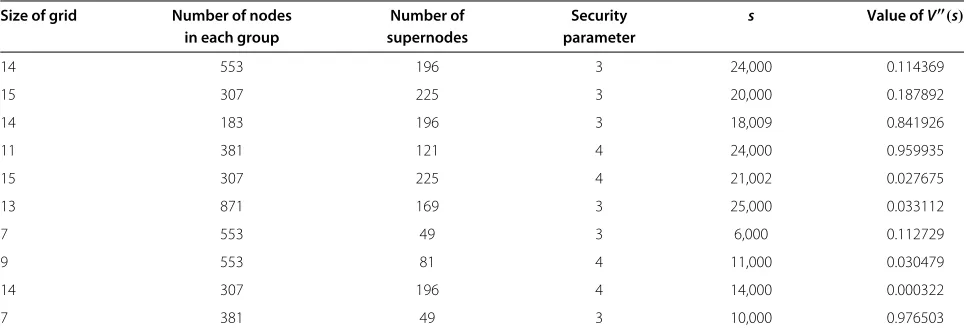
Table 7 gives the values ofV(s)for different values of the number of captured nodes. It can be seen from Table 7 that the value ofV(s)is very low even if a high number of nodes are captured. So, the key predistribution model is highly resilient as far as theV(s) is concerned. Also, if the size of the grid is increased, the value ofV(s)gets reduced.

5.4 Comparison with other schemes

Next, we compare our proposed scheme with some other key predistribution schemes that use deployment knowl-edge. These schemes include Du et al. 2004 [20] and 2006 [21], Liu and Ning 2003 [39] and 2005 [40], Yu and Guan 2005 [28] and 2008 [29], Zhou et al. 2006 [23], Huang et al. [24], Huang and Medhi 2007 [25], Chan and Perrig 2005 [26], Simonova et al. 2006 [27].

Huang et al. [24,25] used rectangular deployment zone which is divided into equal-sized regions of smaller size. In this scheme, the sensors randomly choose the keys. Huang et al. used multispace Blom scheme [4] for key predistri-bution. In this scheme, all nodes are identical with respect

to the amount of resources they possess. This is where this scheme is different from ours. In our scheme, there are two different types of nodes viz. common nodes and agents giving rise to a heterogeneous network. Moreover, in Huang et al. scheme, the nodes in a region can commu-nicate directly with each other with probability of>0.5; whereas, in our scheme, they can do so with a probability equal to 1 as our scheme ensures full interregion connec-tivity. Hence, in this scheme, more amount of computa-tion will be required for communicacomputa-tion than our scheme. The scheme of Huang et al. is perfectly secure against selective and random node capture attack. Hence, cap-ture of some number of nodes by an adversary will have negligible effect to the links among the uncompromised nodes. However, if we take all the links of compromised and uncompromised nodes into account, then the fraction of links compromised will be higher.

Zhou et al. [23] used two types of sensor nodes viz. static and mobile. This scheme uses pairwise keys with each sensor within the same region. Hence, it requires high amount of memory to hold the pairwise keys if the number of sensors within a region is high enough. If there arennumber of nodes within a region, then the number of keys to be stored in a node isO(n2) under the Zhou et al. scheme; whereas, it isO(√n)in Çamptepe and Yener scheme which is used in our key predistribution scheme. Hence, our scheme is much better than Zhou et al. in terms of memory efficiency.

Liu and Ning [39,40] used deployment knowledge. There, the whole deployment zone is split into smaller square regions like our scheme. However, in their schemes, only a single node is deployed in a square region as opposed to our scheme where there are a group of nodes deployed in a region. They used the polynomial-based scheme of Blundo et al. [5]. The deployment region is broken down into equal-sized squares{Cic,ir}ic = 0, 1,. . .,C−1,ir = 0, 1,. . .,R−1 ,

Table 7 Values ofV(s)for different values ofs, size of grid and number of nodes in each group

Size of grid Number of nodes Number of Security s Value ofV(s)

in each group supernodes parameter

14 553 196 3 24,000 0.114369

15 307 225 3 20,000 0.187892

14 183 196 3 18,009 0.841926

11 381 121 4 24,000 0.959935

15 307 225 4 21,002 0.027675

13 871 169 3 25,000 0.033112

7 553 49 3 6,000 0.112729

9 553 81 4 11,000 0.030479

14 307 196 4 14,000 0.000322

each of which is a cell with coordinates(ic,ir)denoting

row ir and column ic . Each of the cells is

associ-ated with a bivariate polynomial. For a R × C grid, the setup server generates RC t-degree polynomials {fic,ir(x,y)}ic = 0, 1,. . .,C − 1,ir = 0, 1,. . .,R − 1, and assigns fic,ir(x,y) to cell Cic,ir. For each sensor, the setup server determine its home cell and its four neighboring cells which lie adjacent to the home cell in the same row and column. The setup server dis-tributes to the sensor the coordinates of the home cell and the polynomial shares of the home cell and its neighboring cell. For example, for a sensor Uu in

the cell with coordinate (r,c), the polynomial shares fr−1,c(u,y),fr,c−1(u,y),fr+1,c(u,y),fr,c+1(u,y),fr,c(u,y)

are given. For direct key establishment, a node broadcasts the coordinates of its home cell. From this coordinate, the destination node finds out the common polynomial that it shares with the broadcasting node if at all. Now, the common key can be calculated using the same method as [5].

In Simonova et al.’s [27] scheme, the number of special-ized nodes depends upon the size of the network unlike ours which is constant (=1). The resiliency as given in the graph is much lower compared to our scheme. Also, resiliency in terms of nodes or regions disconnected has not been presented.

Du et al. [21] proposed another key predistribution using deployment knowledge that uses multiple space Blom scheme [4]. Under this scheme, sensors randomly choose keys from a set of different instances of Blom space. Unlike our scheme, this scheme does not guaranty full connectivity.

As we have discussed earlier, the key predistribu-tion scheme of Ruj and Roy in [18] uses deployment knowledge. Similar to our scheme, this scheme uses

the Çamptepe and Yener scheme for key predistribu-tion within the same region. This scheme exhibits lower resiliency among the set of agents that provide interre-gion connectivity as discussed in previous sections. In other words, our scheme offers more resilient interregion connectivity than Ruj and Roy scheme.

Figure 5 shows a pictorial comparison of our scheme with standard schemes that use deployment knowledge. This comparison is based on the values of fraction of total links broken when some nodes get captured. This com-parison takes into account all the links in the network which includes the links in compromised nodes as well. The parameters of the different schemes are following:

DDHV scheme has parametersk = 200,ω = 11, and τ = 2. LN scheme has parametersk =200,m= 60, and L=1; YG scheme has parametersk =100; ZNR scheme has parametersk=100; HMMH scheme has parameters k=200,ω=27, andτ =3; SLW scheme has parameters k = 16,p= 11, andm= 4; Ruj-Roy scheme has param-eters k = 12. Our scheme has parametersp = 11 and c = 4. The size of the network in DDHV, LN, YG, ZNR, and HMMH is 10,000; for SLW, it is 12,100. It is 16,093 for Ruj-Roy scheme and in our scheme. We simulated the behavior of the key predistribution schemes for random node capture attack. All schemes are implemented iden-tical network. It can be seen in Figure 5 that our scheme offers better performance than similar schemes that make use of deployment knowledge up to a certain limit of the number of nodes captured by the adversary. We used C program for running the simulation.

The reason why our scheme excels in performance can be inferred from Lemma 3 and Proposition 4. Lemma 3 says that in order to compromise the links between any two nodes, the adversary is required to compro-mise at leastc(cis the security parameter) nodes having

0 0.2 0.4 0.6 0.8 1

0 200 400 600 800 1000

F

raction of links e

xposed

Number of nodes compromised

SLW HMMH YG RR LN ZNR DDHV Ours