Thin-sheet electromagnetic inversion modeling using
Monte Carlo Markov Chain (MCMC) algorithm
Hendra Grandis1, Michel Menvielle2, and Michel Roussignol3
1Department of Geophysics and Meteorology, Institut Teknologi Bandung (ITB), Jalan Ganesha 10, Bandung - 40132, Indonesia 2Centre d’Etude des Environnements Terrestre et Plan´etaires, 3, Avenue de Neptune, F-94107 Saint Maur des Fosses, France 3Equippe d’Analyse et de Math´ematique Appliqu´ee, Universit´e de Marne la Vall´ee, 5, Boulevard Descartes, F-77454 Marne la Vall´ee, France
(Received November 20, 2000; Revised February 13, 2002; Accepted February 13, 2002)
The well-known thin-sheet modeling has become a very useful interpretation tool in electromagnetic (EM) methods. The thin-sheet model approximates fairly well 3-D heterogeneities having a limited vertical dimension. This type of approximation leads to amenable computation of EM response of a relatively complex conductivity distribution. This paper describes the integration of thin-sheet forward modeling into an inversion method based on a stochastic Monte Carlo Markov Chain (MCMC) algorithm. Effective exploration of the model space is performed using a biased sampler capable to avoid entrapment to local minima frequently encountered in a such highly non-linear problem. Results from inversion of synthetic EM data show that the algorithm can reasonably resolve the true structure. Effectiveness and limitations of the proposed inversion method is discussed with reference to the synthetic data inversions.
1.
Introduction
The thin-sheet modeling has proven to be an effective tool for the interpretation of electromagnetic (EM) data, espe-cially when heterogeneities are confined in a layer having limited vertical dimension. The thin-sheet approximation is valid if the thickness of the thin layer containing hetero-geneities is much smaller than the penetration depth of EM fields. The model is then represented by lateral variations of conductance, i.e. integrated conductivity over the thickness of the thin layer. This approximation significantly simpli-fies the resolution of the Maxwell’s equations describing the EM fields in quasi three-dimensional (3-D) media. There are several working algorithms employing integral equation method for thin-sheet EM modeling (e.g. Vasseur and Wei-delt, 1977; McKirdyet al., 1985) and their advanced ver-sions as reported by Wang and Lilley (1999, and references therein).
An inversion scheme devised to resolve strongly non-linear problems, such as those in EM methods, has been re-cently proposed by Grandiset al.(1999, 2002). The inverse problem recast in the Bayesian inference approach is solved by using a stochastic Monte Carlo Markov Chain (MCMC) algorithm. The method has been successfully applied to 1-D magnetotelluric (MT) modeling for both synthetic and real data as well (Grandis, 1997; Grandiset al., 1999). Similar approach applied to thin-sheet EM modeling also gave en-couraging results (Jouanne, 1991; Roussignolet al., 1993). In the latter, Markov chains were used not only to update the model but also to estimate the electric field as iteration
pro-Copy right c The Society of Geomagnetism and Earth, Planetary and Space Sciences (SGEPSS); The Seismological Society of Japan; The Volcanological Society of Japan; The Geodetic Society of Japan; The Japanese Society for Planetary Sciences.
gresses. The convergence of the modified (or 2-D) Markov chain has been proven empirically only for cases in which a resistive heterogeneity is contained in a more conductive host layer.
We have incorporated the thin-sheet forward modeling scheme of Vasseur and Weidelt (1977) in our inversion algo-rithm for its simplicity in handling variable exchange (input and output) between forward and inverse part of the algo-rithm. We will first describe the inversion algorithm and also outline the approach adopted by Jouanne (1991) and Roussignolet al.(1993). Then, a modification of the algo-rithm is proposed in order to overcome difficulties encoun-tered in the previous approach. The modification consists in a quasi-complete resolution of the electric field involved in the forward modeling calculation. The method was tested to invert synthetic data corresponding to simple resistive (or conductive) structure in a conductive (or resistive) host. A special attention has been paid to the resolving capability of the method faced to particularities of EM data (i.e. MT impedance tensor and induction vector) and also to different discretization of prior conductance.
2.
MCMC Inversion Algorithm
For completeness, we will describe the non-linear inver-sion method based on MCMC algorithm focusing mainly on practical aspects of the method in order to illustrate more clearly how the algorithm works. The readers are referred to Grandis et al. (1999, 2002, and references therein) for theoretical details of the method.
In the Bayesian perspective, resolving an inverse problem can be stated as updating oura prioribeliefs on the model by using information acquired from observations which re-sults in a posterioriknowledge on the model sought. The
Bayesian approach naturally integrates uncertainties of the information involved by using probability density function (pdf) representation (Robert, 1992). For discrete (or discretized) quantities appropriate for our problem, the Bayesian formula takes the following form
p(m|d)=2 g(d|m)h(m)
m∈Eg(d|m)h(m)
(1)
wheredandmdenote data and model vector respectively. In Eq. (1), the posterior probability is represented by the con-ditional probability for the model given the data p(m | d) which in fact is the solution to the inverse problem. The con-ditional probability of the data for a given modelg(d | m) combines both statistics of the data and the resolution of the forward problem whileh(m)is the probability of the prior model. We are usually more interested in the probability for each (or for a certain) model parameter regardless of other model parameters. This marginal posterior probability of a model parametermiis obtained from Eq. (1) by taking inte-gral (or sum in our discrete case) over other model parame-tersmj=isuch that
Significance of this marginal posterior probability of a model parameter will be explained in the subsequent para-graphs.
The denominator of Eqs. (1) and (2) is in fact a normal-izing constant and it sums over the entire possible models in the model space. For a model consisting of M model parameters, i.e.m =[mi] (i = 1,2, . . . ,M), and thei-th model parameter can takeNidiscrete possible (prior) values
ρj (j = 1,2, . . . ,Ni) then the number of possible mod-els in E is the product of N1 × N2 × · · · × NM. For a
homogeneous parameterization used in our case the num-ber of possible (prior) values is the same for each model parameter. Then the number of possible models in E is NM. However in any case, numerical computation of (1) or (2) is impractical or even impossible for most geophys-ical problems having a large number of model parameters and complicated non-linear forward problem. A stochastic algorithm is then formulated to efficiently sample the model space. Unlike pure Monte Carlo methods which sample ran-domly the model space with uniform probabilities, the Gibbs sampler used in the algorithm employs a certain conditional probability to bias the sampling process such that regions having significant contribution to the posterior pdf are sam-pled efficiently.
Consider a case in which model parameters other thanmi are fixed to their actual (or most recent) value. Then, we have a conditional posterior probability for model parameter migiven other model parametersmj=ifixed, i.e.
ˆ
In the above equation we explicitly state thatmi can take
ρk; k = 1,2, . . . ,N as its value such that pˆ(mi = ρk |
d) ≡ f(ρk), which is also applicable for p(mi | d). The difference is that in Eq. (2) we have to consider all possible values formj=iand sum the probabilities associated to them, while in Eq. (3) only probabilities related to actual values for mj=i are concerned. The normalizing constant in Eq. (3) involves a sum over all possible values for the model parameters such that it can be amenable for a reasonable number ofN.
The importance of the conditional posterior probability for a model parameter given in Eq. (3) will be evident by making it more explicit. By establishing d = [di] i = 1,2, . . . ,N Das observational data, theng(d|m)is com-monly called likelihood function (Jackson and Matsu’ura, 1985; Sen and Stoffa, 1996). We consider that data errors are independent and obey a Gaussian distribution with zero mean and varianceσ2so that the likelihood function can be
written as from an application of the forward modeling operatorFand C retains all constants involved. Substituting Eq. (4) to Eq. (3) by further assuming a homogeneous probability for the prior model results in a more explicit formula as follows
ˆ
whereC again absorbs all normalizing constants including the denominator of Eq. (3). For a fixedmj=i Eq. (5) rep-resents relative probabilities of ρk (k = 1,2, . . . ,N) as possible values for mi. Thus, Eq. (5) can be utilized to update mi by using a value drawn from ρk weighted by
ˆ
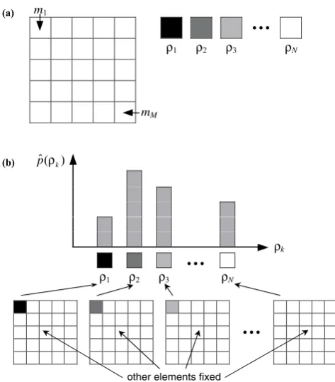
p(mi =ρk |d);k=1,2, . . . ,N. It’s obvious thatρk cor-responding to a smaller misfit will have a greater probability to be selected. However, values with greater misfit still have a chance to be selected, they are only less probable. The latter gives the algorithm an ability to escape local minima frequently encountered in strongly non-linear inverse prob-lems. Figure 1 illustrates the model parameterization used in the Markov chain algorithm and how the conditional pos-terior probability is used to update a model parameter.
(a) m1
Fig. 1. A schematic diagram illustrating (a) model parameterization and (b) selection of prior values to update a parameter model using the conditional posterior probability.
have been discussed in detail by Rothman (1986). Here, we only exploit their practical consequences. After suffi-ciently a long time the Markov chain exhibits a stationary state—independent of its initial state—described by its in-variant probability. It has been shown (see e.g. Grandiset al., 1999, 2002) that the invariant probability of the con-structed Markov chain is in fact the posterior probability defined in Eq. (1). Further theorem on asymptotic behav-iors of the Markov chain implies that in general empirical averages tend towards statistical averages (Heerman, 1990; Robert, 1996). This in turn simplifies the evaluation of pos-terior quantities, especially the marginal pospos-terior probabil-ity from which statistical measures for a model parameter (mean and variance) can be estimated.
3.
Thin-Sheet Inversion Algorithm
In the thin-sheet modeling, calculation of the electric field is performed by discretizing the thin layer containing hetero-geneities into rectangular uniform cells. The conductance of each cell is assumed constant. By using the integral equation method, the computation domain covers only the anomalous zone where the conductance differs from that of normal host medium. The electric field is then used to calculate the mag-netic field to obtain theoretical or calculated EM transfer functions (i.e. MT impedance tensor and magnetic transfer function).
The total electric field in thek-th cell located at the hetero-geneous layer is expressed by (Vasseur and Weidelt, 1977)
E(k)=En(k)−iωμ0
"
k∈K
τkG(k,k)·E(k), (6)
whereEn(k)is the normal electric field associated with
nor-mal (stratified or 1-D) conductivity distribution,G(k,k)is the Green kernel representing electric field atkdue to a uni-tary dipole atkandτk denotes anomalous conductance of thek-th cell,k,k ∈ K. Equation (6) is in fact a system of N =2K linear equations associated to orthogonal electric fields (Ex,Ey) at each cell corresponding to a certain con-ductance distribution. However, in the subsequent equations the vector representation of the electric field is retained for the sake of clarity.
For a large number of cells in the anomalous domain, a direct matrix inversion to resolve (6) is prone to round-off errors and instability and may require a considerable com-puter memory. Additionally, the form of Eq. (6) is such that it is more suitable to use the iterative Gauss-Seidell method in which an initial value of the solution is updated iteratively to obtain the solution (Jainet al., 1987). A particular char-acteristic of the Gauss-Seidell method is the use of updated elements of the solution to estimate the remaining elements. At(j+1)-th iteration, the estimated electric field is calcu-lated by
where the normal electric field is constant throughout the iteration process. To accelerate convergence we use an over-relaxation parameterwsuch that
E(k)j+1=E(k)j+w(Eˆ(k)j+1−E(k)j). (8)
The normal electric field En(k) is commonly used as the initial value forE(k)0and in general convergent solution is
obtained after 10 to 20 iterations, as long as the conductivity contrast is not too high (Vasseur and Weidelt, 1977).
In order to reduce the computation time of the forward modeling, Jouanne (1991) and Roussignol et al. (1993) adopted a 2-D Markov chain approach to simultaneously es-timate the conductance and the electric field of a cell. At a given step (i.e. conductance change of the k-th cell), the electric field at k-th cell is computed by performing one (incomplete) Gauss-Seidell iteration based on previous step values using Eqs. (7) and (8). The electric field in all other cells different thankis computed to account for the change of conductance and electric field in thek-th cell by using
E(k)j+1 =E(k)j+[(τk)j+1−(τk)j]E(k)j+1 (9)
wherek = k. This is an approximation that neglects sec-ondary effect at cells different than k and k produced by changes of electric field and conductance in k-th cell. The pair (mj,Ej) constitutes, in effect, a Markov chain since it depends on their past states only through (mj−1,Ej−1).
0 5 10 15
G-S ITERATION
0.0 1.0 2.0 3.0
Δ
En
(a)
0.0 1.0 2.0 3.0
Δ
0 5 10 15
G-S ITERATION
En
(b)
resistive
conductive resistive
conductive
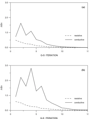
Fig. 2. Convergence curves of the electric field calculation corresponding to two different resistivity contrast between host and anomalous zone: (a) 10:500 Ohm.m and (b) 5:500 Ohm.m. It is shown that convergence is more difficult to attain and is slower for the conductive anomaly.
data showed that the chain is convergent for resistive het-erogeneities in a conductive thin layer and the true or syn-thetic models were fairly well resolved. In the case where the heterogeneity is more conductive than the host medium, the Markov chain diverges (Jouanne, 1991; Roussignolet al., 1993). From practical point of view, the above facts ex-clude the application of inversion method using the Markov chain algorithm in the majority of interesting real situations where heterogeneities are mainly conductive in a more resis-tive environment. From theoretical point of view, empirical convergence of the Markov chain only for a certain class of models does not guarantee that it will be the case for every model in that class due to absence of mathematical proof. Therefore, convergence of the Markov chain must be estab-lished empirically for every class of models considered.
The assessment of the convergence of the forward mod-eling algorithm was performed by using synthetic models in order to identify possible causes of difficulties in resolving conductive anomalies in a resistive host. For a given con-ductance distribution in the thin-sheet and the stratified host medium, the resolution of the forward modeling is based on the calculation of the electric field at the thin-sheet. The
probabil-10 Ohm.m or 500 Ohm.m 5 km
500 Ohm.m 40 km
1000 Ohm.m 70 km
10 Ohm.m
z (arbitrary scale)
surface
(b)
host medium
anomalous zone
y (east) x (north)
(a)
30 km
Fig. 3. Synthetic model: (a) geometry of the anomalous zone in the thin-sheet and (b) stratified or 1-D host medium containing the thin-sheet.
ρYX
ρXY
ρYX
ρXY
0 10 20 50 100 200 500 1000
APP. RESISTIVITY (Ohm.m)
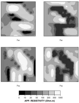
Fig. 4. Apparent resistivity maps calculated from principal components of the impedance tensor (ρx yandρyx) forT=1000 sec., resistive anomaly (left) and conductive anomaly (right).
ity for the Markov chain. This in turn leads to convergence problem of the Markov chain especially in the case of con-ductive structure in a resistive host.
The Markov chain algorithm relies on the transition prob-ability (5) such that if its precision is insufficient, it will lead to difficulty in generating convergent and optimal models. Therefore, we propose to modify the existing Markov chain algorithm to overcome the above limitations. The
real part
imaginary part
0.25
0.25
real part
imaginary part
0.125
0.125
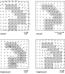
Fig. 5. Induction arrow map showing real and imaginary parts forT=1000 sec. of the resistive anomaly (left) and the conductive anomaly (right).
fact, we need to resolve only partially the system of equa-tions defining the electric field in the calculation of the tran-sition probability. The Markov chain is supposed to be con-vergent in practically all situations (i.e. conductivity config-uration of the anomalous zone and the host medium) as long as the forward modeling is also convergent. In this case, the Markov chain retains its 1-D character as described in Section 2, i.e. it has only one discrete variable which is the conductance of the thin-sheet.
4.
Inversion of Synthetic Data
4.1 Synthetic model and synthetic dataIn this study, synthetic thin-sheet models corresponding to a regional or large scale environment were used to gen-erate synthetic data. The typical 1-D model consists of four layers having resistivities of 10 or 500 Ohm.m, 500 Ohm.m, 1000 Ohm.m and 10 Ohm.m with thickness of 5, 40, 70 km respectively. The thin-sheet is the uppermost or surface layer and the resistivity contrast between anomalous zone and the normal host is 500 to 10 Ohm.m which correspond to a contrast in conductance of 10 to 500 Siemens (i.e. a resistive structure embedded in a conductive layer). For a conductive structure embedded in a resistive layer, resistiv-ities are simply interchanged. In the subsequent paragraphs we denote the two cases by the anomalous zone, i.e. resistive anomaly and conductive anomaly. The thin-sheet containing the anomalous zone is divided into 10×10 cells, each has 30 km wide. Outside that zone the medium is 1-D as described above (Fig. 3).
At the center of each cell we calculated the electric and magnetic fields due to conductivity configuration in the syn-thetic model described above. The EM fields components are in the orthogonal coordinate system commonly adopted in the geomagnetic studies, i.e. x positive to the North, y positive to the East andzpositive downwards. The periods used (300, 1000, 3600 and 7200 seconds) and the layer dis-cretization are such that the thin-sheet approximation holds. The complex transfer functions common to EM studies (i.e. impedance tensor and magnetic transfer function or induc-tion vector) were then calculated according to the following well-known relations
Ex Ey
=
Zx x Zx y Zyx Zyy
Hx Hy
or E=Z·H, (10)
Hz=TzxHx+TzyHy. (11)
Table 1. Quasi-linearly discretized prior conductances (50 Siemens interval except for values lower than 50 Siemens) with their corresponding resistivity values and anomalous conductance relative to normal conductance for resistive and conductive anomalies.
Conductance Resistivity Anomalous conductance (Siemens)
(Siemens) (Ohm.m) Resistive anomaly Conductive anomaly
1.0 5000.0 −499.0 −9.0
10.0 500.0 −490.0 0.0
50.0 100.0 −450.0 40.0
100.0 50.0 −400.0 90.0
150.0 33.3 −350.0 140.0
200.0 25.0 −300.0 190.0
250.0 20.0 −250.0 240.0
300.0 16.7 −200.0 290.0
350.0 14.3 −150.0 340.0
400.0 12.5 −100.0 390.0
450.0 11.1 −50.0 440.0
500.0 10.0 0.0 490.0
550.0 9.1 50.0 540.0
600.0 8.3 100.0 590.0
Table 2. Quasi-logarithmically discretized prior conductances with their corresponding resistivity values and anomalous conductance relative to normal conductance for resistive and conductive anomalies.
Conductance Resistivity Anomalous conductance (Siemens)
(Siemens) (Ohm.m) Resistive anomaly Conductive anomaly
1.0 5000.0 −499.0 −9.0
2.0 2500.0 −498.0 −8.0
5.0 1000.0 −495.0 −5.0
10.0 500.0 −490.0 0.0
20.0 250.0 −480.0 10.0
50.0 100.0 −450.0 40.0
100.0 50.0 −400.0 90.0
200.0 25.0 −300.0 190.0
500.0 10.0 0.0 490.0
1000.0 5.0 500.0 990.0
2000.0 2.5 1500.0 1990.0
5000.0 1.0 4500.0 4990.0
real and imaginary induction arrows according to the fol-lowing convention
¯
VRe= −Re(Tzx)xˆ−Re(Tzy)yˆ, (12a)
¯
VIm=Im(Tzx)xˆ+Im(Tzy)yˆ. (12b)
wherexˆandyˆare unitary vector in thex- andy-axes respec-tively. Note that the direction of the real induction vector is inverted such that it conforms to the Parkinsons induction ar-rows. With this convention, the real induction arrows point towards the conductive medium (Fig. 5). From Figs. 4 and 5 we can observe relative sensitivities of different impedance tensor components and also different types of data (appar-ent resistivity or real and imaginary parts of the induction
arrows) related to the form of the anomaly. This may indi-cate which characteristic feature of the model than can be inferred from these different type of data in the qualitative interpretation. For example, it is well known that appar-ent resistivity map reveals more clearly conductivity con-trast perpendicular to the electric field direction (TM mode) and so forth.
4.2 Prior model
uni-(c) (d)
(a) (b)
1 10 50 100 150 200 250 300 350 400 450 500 550 600
CONDUCTANCE (Siemens)
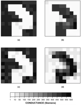
Fig. 6. Conductance map obtained from inversion using linear discretization of prior conductance values: inversion of impedance tensor for (a) resistive and (b) conductive anomaly, inversion of induction vector for (c) resistive and (d) conductive anomaly.
form pdf for prior conductances in a given interval cover-ing the anomalous and normal conductance values. In this interval, a set of discrete conductance values were used as prior or possible values for the model parameter (conduc-tance of each cell). The discretization interval of possible conductance values may substantially dictate the inversion results. Therefore, we used two kinds of discretization, i.e. quasi-linear and quasi-logarithmic discretizations (see Ta-bles 1 and 2) to evaluate their influence on the sensitivity of the inversion algorithm and also on the marginal posterior probability of the model parameters. Note that in Tables 1 and 2 anomalous conductance signifies conductance differ-ence of a cell or a block relative to the conductance of the host or normal thin-layer. In subsequent paragraphs, quasi-linear and quasi-logarithmic discretization of prior conduc-tance will be termed simply linear and logarithmic prior con-ductance values.
4.3 Results
A number of inversions were performed using both lin-ear and logarithmic prior conductance values with the ten-sor impedance and induction vector as the data. Prelimi-nary tests showed that the convergence was obtained after 5 to 10 iterations after which posterior values (marginal pdf and model parameters) oscillate around their optimum val-ues. Inversions are systematically effected up to 20
itera-tions and results of the last 15 iteraitera-tions were averaged. Fig-ures 6 and 7 show the inversion results using linear and log-arithmic prior conductance values respectively. The results are presented as maps representing conductance distribution in the thin-sheet. In general, the true structure can be re-solved fairly well, except in the case of inversion of induc-tion vector for conductive anomaly (Figs. 6(d) and 7(d)). In the latter, the result probably stems from the fact that a con-ductive anomaly confined in a resistive host produces a low magnitude anomaly, especially in terms of induction vector (Menvielleet al., 1982). Therefore, poor resolution of this type of anomaly is mainly related to the type of data since the same conductive anomaly is more clearly resolved from inversion of the impedance tensor (Figs. 6(b) and 7(b)).
(c) (d)
(a) (b)
1 2 5 10 20 50 100 200 500 1000 2000 5000
CONDUCTANCE (Siemens)
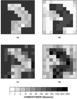
Fig. 7. Conductance map obtained from inversion using logarithmic discretization of prior conductance values: inversion of impedance tensor for (a) resistive and (b) conductive anomaly, inversion of induction vector for (c) resistive and (d) conductive anomaly.
different discretization of prior conductance leads to dif-ferent effect on the resolution of resistive and conductive zones. In case of linear prior conductance values, the in-version algorithm is able to differentiate 1, 10, 50 and 100 Siemens and to choose the true value (10 Siemens) for re-sistive zones. For conductive zones, the inversion method has difficulty to distinguish conductance values between 350 and 600 Siemens in 50 Siemens interval. In case of logarith-mic prior conductance values, conductive zones appears to be better resolved due to a large difference in prior conduc-tance values for the conductive interval (100, 200, 500 and 1000 Siemens).
By assuming that the thickness of the thin-sheet is known, linear prior conductance values for resistive zones are ob-viously different expressed in terms of resistivity, i.e. 5000, 500, 100, 50 Ohm.m. For conductive zones, linear prior con-ductance corresponds to resistivities between 8 to 15 Ohm.m which are imperceptible in the inversion. In this interval, a conductive zone can be characterized by any resistivity value. The same explanations are also valid for logarithmic prior conductance values (see Table 2).
The transition probability of the Markov chain at the last (20-th) iteration supports more clearly the facts described in the above paragraph. The transition probability is theoreti-cally convergent to the marginal posterior probability of the
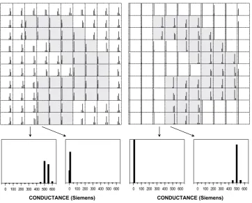
model parameters, although the latter is generally better esti-mated using empirical average of the transition probabilities (Grandiset al., 1999; Schottet al., 1999). In the following only results from inversion of the impedance tensor are pre-sented. Figure 8 presents the transition probability of each model parameter at the last iteration for linear prior conduc-tance values. The probability is represented as histogram plotted at each cell where the horizontal axis is the conduc-tance scale. A zoom of the transition probability for two adjacent cells indicated by arrows is also shown in Fig. 8. The same set of figures for logarithmic prior conductance values are presented in Fig. 9. A well resolved model pa-rameter is characterized by a nearly single bar at or around the true conductance value (i.e. resistive at the left side of each cell). In contrast, a less well resolved model parame-ter may be identified from nearly uniform small bars around the true conductance value (i.e. conductive at the right side of each cell). Similar results were also obtained from inver-sion of the induction vector data.
5.
Conclusion
0 100 200 300 400 500 600 0 100 200 300 400 500 600 0 100 200 300 400 500 600 0 100 200 300 400 500 600
CONDUCTANCE (Siemens) CONDUCTANCE (Siemens)
Fig. 8. Histogram representing transition probability at the last (20-th) iteration of each cell for linear discretization of prior conductance values: inversion of impedance tensor for resistive (left) and conductive anomaly (right). A zoom of the transition probability for two adjacent cells indicated by arrows is shown below each figure.
1E-1 1E+0 1E+1 1E+2 1E+3 1E+4 1E-1 1E+0 1E+1 1E+2 1E+3 1E+4 1E-1 1E+0 1E+1 1E+2 1E+3 1E+4 1E-1 1E+0 1E+1 1E+2 1E+3 1E+4
CONDUCTANCE (Siemens) CONDUCTANCE (Siemens)
recognize that approximate estimation in the calculation of the Markov chain’s transition probability was inadequate, especially for conductive anomalies. This leads to an idea of incorporating more Gauss-Seidell iterations in the calcu-lation of the forward modeling such that more accurate esti-mate of the transition probability is obtained. The modified inversion algorithm is thus applicable to invert data corre-sponding to both resistive and conductive anomaly as well. From theoretical point of view, the modification also pre-serves one-dimensional Markov chain for which mathemar-tical proof of convergence has been established (Grandis, 1994, 2002).
The effectiveness of the algorithm was tested by perform-ing inversions of synthetic data in the form of impedance tensor and induction vector. In general, synthetic models containing resistive and conductive anomalies are fairly well resolved. Best results were obtained from inversion of the MT impedance tensor data suggesting that these kind of data provide more information on the conductivity distribution in the thin-sheet. Different discretization of prior conduc-tance values revealed that, for a given thickness of the thin-sheet, the inversion algorithm is more sensitive to resistivity value of the thin-sheet. Thus, in discretizing prior conduc-tance we have to consider the corresponding resistivity val-ues such that the inversion can resolve both resistive and conductive anomalies equally well with a reasonable resolu-tion. This implies that the thickness of the thin-sheet must be relatively well knowna priori. Provided that thisa pri-oriinformation is known, a possible strategy in applying the inversion method to real data consists of (i) inversion us-ing a coarse prior conductance values in a large interval to identify predominant anomalies, and (ii) inversion using a finer discretization of prior conductance around these pre-dominant anomalies. Such strategy is necessary to obtain a good model resolution while keeping reasonable compu-tational time by using a relatively limited number of prior conductance values. Note that the number of prior conduc-tance values corresponds to the number of forward modeling in each step of the algorithm, i.e. calculation of the transition probability used to update a model parameter.
The proposed inversion method belongs to global search and gradient-free optimization methods which can effec-tively overcome difficulties of local search or linearized ap-proach of strongy non-linear problems. The MCMC algo-rithm is, in general, computer intensive and slow since a large number of forward modeling has to be effected to re-solve the inverse problem. However, more informative solu-tion in terms of marginal posterior pdf of the model parame-ters represent invaluable information in assessing the uncer-tainty and, to some extent, the non-uniqueness of the solu-tion (Sen and Stoffa, 1996). For cases in which the pdf of the model parameters is not Gaussian nor unimodal (which is the case for most non-linear problems), standard estimators (i.e. mean and variance) would be severely biased and even
meaningless in the worst cases (Taritset al., 1994). It is then important to base our interpretation of the inverted models directly using the marginal posterior pdf of the model pa-rameters.
Acknowledgments. The authors greatly acknowledge Pascal Tarits and Virginie Jouanne for fruitful discussions during the preparation of this paper.
References
Grandis, H., Imagerie electromagnetique Bayesienne par la simulation d’une chaˆıne de Markov, Ph.D. thesis, Universit´e Paris 7, 278 pp., 1994. Grandis, H., Application of magnetotelluric (MT) method in mapping base-ment structures: Example from Rhine-Saone Transform Zone, France, Indonesian Mining Journal,3, 16–25, 1997.
Grandis, H., M. Menvielle, and M. Roussignol, Bayesian inversion with Markov chains—I. The magnetotelluric one-dimensional case,Geophys. J. Inter.,138, 757–768, 1999.
Grandis, H., M. Menvielle, and M. Roussignol, Monte Carlo Markov Chains for non-linear inverse problems: an algorithm,Mathematical Ge-ology, 2002 (submitted).
Heerman, D. W., Computer simulation methods in theoretical physics, Springer-Verlag, Berlin, 1990.
Jackson, D. D. and M. Matsu’ura, A bayesian approach to nonlinear inver-sion,J. Geophys. Res.,90(B1), 581–591, 1985.
Jain, M. K., S. R. K. Iyengar, and R. K. Jain, Numerical methods for scientific and engineering computation, Wiley Eastern, 1987.
Jouanne, V., Application des techniques statistiques bayesiennes `a l’inver-sion de donn´ees ´electromagn´etiques, Ph.D. thesis, Universit´e Paris 7, 1991.
McKirdy, D. McA., J. T. Weaver, and T. W. Dawson, Induction in a thin sheet of variable conductance at the surface of a stratified earth—II: Three-dimensional theory, Geophys. J. Roy. astr. Soc., 80, 177–194, 1985.
Menvielle, M., J. C. Rossignol, and P. Tarits, The coast effect in terms of deviated electric currents: a numerical study,Phys. Earth Planet. Inter., 28, 118–128, 1982.
Robert, C.,L’analyse Statistique Bayesienne, 393 pp., Economica, Paris, 1992.
Robert, C.,Methodes de Monte Carlo par Cha´ ˆınes de Markov, 393 pp., Economica, Paris, 1996.
Rothman, D. H., Automatic estimation of large residual statics corrections, Geophysics,51, 332–346, 1986.
Roussignol, M., V. Jouanne, M. Menvielle, and P. Tarits, Bayesian electro-magnetic imaging, inComputer Intensive Methods, edited by W. Hardle and L. Siman, pp. 85–97, Physical Verlag, 1993.
Schott, J.-J., M. Roussignol, M. Menvielle, and F. R. Nomenjahanary, Bayesian inversion with Markov chains—II. The one-dimensional DC multilayer case,Geophys. J. Inter.,138, 769–783, 1999.
Sen, M. K. and P. L. Stoffa, Bayesian inference, Gibbs’ sampler and un-certainty estimation in geophysical inversion,Geophys. Prosp.,44, 313– 350, 1996.
Tarits, P., V. Jouanne, M. Menvielle, and M. Roussignol, Bayesian statistics of non-linear inverse problems: examples of the magnetotelluric 1-D inverse problem,Geophys. J. Inter.,119, 353–368, 1994.
Vasseur, G. and P. Weidelt, Bimodal electromagnetic induction in non-uniform thin sheets with an application to the northern Pyrenean induc-tion anomaly,Geophys. J. Roy. astr. Soc.,51, 669–690, 1977.
Wang, L. J. and F. E. M. Lilley, Inversion of magnetometer array data by thin-sheet modeling,Geophys. J. Inter.,137, 128–138, 1999.