R E S E A R C H
Open Access
Time-frequency optimization for
discrimination between imagination of right
and left hand movements based on two
bipolar electroencephalography channels
Yuan Yang
1,4, Sylvain Chevallier
2, Joe Wiart
3,4and Isabelle Bloch
1,4*Abstract
To enforce a widespread use of efficient and easy to use brain-computer interfaces (BCIs), the inter-subject robustness should be increased and the number of electrodes should be reduced. These two key issues are addressed in this contribution, proposing a novel method to identify subject-specific time-frequency characteristics with a minimal number of electrodes. In this method, two alternative criteria, time-frequency discrimination factor (TFDF) andFscore, are proposed to evaluate the discriminative power of time-frequency regions. Distinct from classical measures (e.g., Fisher criterion,r2coefficient), the TFDF is based on the neurophysiologic phenomena, on which the motor imagery BCI paradigm relies, rather than only from statistics.Fscore is based on the popularFisher’sdiscriminant and purely data driven; however, it differs from traditional measures since it provides a simple and effective measure for quantifying the discriminative power of a multi-dimensional feature vector. The proposed method is tested on BCI competition IV datasets IIa and IIb for discriminating right and left hand motor imagery. Compared to state-of-the-art methods, our method based on both criteria led to comparable or even better classification results, while using fewer electrodes (i.e., only two bipolar channels, C3 and C4). This work indicates that time-frequency optimization can not only improve the classification performance but also contribute to reducing the number of electrodes required in motor imagery BCIs.
Keywords: Brain-computer interface; Electroencephalography; Time-frequency analysis; Electrode reduction; Feature extraction
1 Introduction
After several decades of development, current brain-computer interface (BCI) systems can now be driven based on various types of brain signals obtained by techniques such as electroencephalography (EEG) [1], functional magnetic resonance imaging (fMRI) [2], near-infrared spectroscopy (NIRS) [3], etc. Thanks to its low-cost, non-invasivity, and high temporal resolution, the scalp EEG is a popular technique for BCIs [1]. One typical paradigm of EEG-based BCI is motor imagery BCI, which classifies subject’s motor intention based on the spatial difference of EEG patterns. The underlying physiological
*Correspondence: Isabelle.Bloch@telecom-paristech.fr
1Institut Mines-Telecom, Telecom ParisTech/CNRS LTCI, 46 rue Barrault, Paris 75013, France
4Whist Lab, Paris 75020, France
Full list of author information is available at the end of the article
phenomenon is that motor imagery of a specific body part (e.g., left hand) induces an event-related desynchroniza-tion (ERD) and/or synchronizadesynchroniza-tion (ERS) in theμandβ bands over the corresponding functional area in the sen-sorimotor cortex [4]. Thus, the essential task of a motor imagery BCI is to extract the task-relevant ERD/ERS pat-terns from EEG signals for classifying subject’s motor intentions.
However, poor signal-to-noise ratio (SNR) of raw EEG signal and mixture of different EEG rhythms (e.g.,αand μrhythms) make it difficult to extract ERD/ERS features for BCI classification [5]. One popular solution is to apply a data-driven spatial filtering technique, such as com-mon spatial pattern (CSP) [6], on multi-channel (e.g. 64 or 128 channels) monopolar recording EEG data, which can improve the SNR of signal and extract discrimina-tive features from the mixture of signals, especially for
two-class discriminations [7]. But such a multi-channel setting inevitably reduces the portability and practicability of BCIs, which represents a main drawback for end users. Thus, bipolar recordings are recommended in portable BCI systems to reduce the number of electrodes [8,9]. A bipolar channel of EEG is obtained by subtracting two monopolar EEG signals [10]. This acquisition improves the SNR by eliminating shared artifacts between two monopolar channels (for details, see [9]). Therefore, they may achieve as good performances as usual multi-channel monopolar settings, using only a few electrodes (i.e., two or three pairs of active electrodes) placed around task-relevant sensorimotor areas. The positions of electrodes in bipolar recording can be optimized algorithmically or using prior knowledge on the spatial location of brain activity during motor imagery [9]. Typically, the bipolar electrodes are placed on locations C3 and C4 of the inter-national 10-20 system [11] (see Figure 1) for hand-related motor imagery tasks since these places correspond to the hand representation areas in the cerebral cortex [12].
However, ERD/ERS patterns are typically short-lasting (half to few seconds) and their frequency range may vary with subjects [13]. Thus, only optimizing the position of electrodes may not be sufficient to achieve a good
Figure 1Positions of C3 and C4.This figure shows positions of C3 and C4 (indicated by ellipses) according to the international 10-20 system [11].
classification, and a BCI system using bipolar recording also requires more precise user-specific time-frequency parameterization in the feature extraction step. To address this problem, a number of approaches were proposed to estimate time-frequency characteristics of motor imagery EEG [13-16], but only a few were successfully applied to bipolar recording data. Among those methods, the fil-ter bank CSP (FBCSP) method seems to be the most effective one, yielding the best BCI performances on BCI competition datasets [17]. FBCSP was initially proposed only for frequency band optimization and then extended to include an optimal temporal selection process [14]. However, FBCSP-based methods involve feature selection procedures based on mutual information, which require tedious iterative steps that greatly increase their com-plexity. Moreover, the latest version of FBSCP selects the optimal time segment from only a few different options, which did not yield better results on bipolar recording data (BCI competition IV dataset IIb) compared to previ-ous versions [14].
methods, is performed on a standard bipolar dataset (the BCI competition IV IIb), and their contribution to elec-trode reduction is evaluated on BCI Competition IV IIa dataset.
2 Time-frequency optimization for classification The EEG signals at C3 and C4 (see Figure 1) are decom-posed into signal components first, in a series of overlap-ping time-frequency regions(ωm×τn),m∈ {1, ,. . .,M}, n ∈ {1,. . .,N} with different frequency bands ωm = [fm,fm+F−1] ,fm+1=fm+Fs(Fis the bandwidth,Fsis the frequency step), and time intervalsτn =[tn,tn+T− 1] ,tm+1=tm+Ts(Tis the interval width,Tsis the time step). The aim of time-frequency optimization is to find a time-frequency region that contains the most discrimina-tive information, so-called the region of interest (ROI), for a given subject. The selected ROI is then used to extract key features for classification.
A measure evaluating the discriminative power of a region should be defined as an increasing function of the discriminative power. This criterion is denotedS. The best ROI(ω∗×τ∗)is estimated by exhaustively searching the largest value ofS(ωm,τn)among all regions:
S(ω∗,τ∗)=max{S(ωm,τn)|m∈{1, 2,. . .,M},n∈ {1, 2,. . .,N}}
(1)
The exhaustive search is reasonable with the chosen val-ues of M and N (1,224 regions in our experiments, as detailed in the next section).
The authors in [20] have reviewed the popular mea-sures, such as Fisher criterion,t-scaled difference,r2 coef-ficient, which are often used in feature selection for BCI systems. However, those measures are typically used for quantifying the discriminative power of one-dimensional feature and are not appropriate for multi-dimensional feature vector evaluation, in particular for our time-frequency optimization. Thus, two novel criteria, TFDF andF score, are designed to address this problem. Dif-ferent from those statistical measures often used in BCIs, TFDF is based on neurophysiological background rather than only statistical distribution of features. F score is based on the popular Fisher’s discriminant, which can be considered as an extended version of Fisher criterion, but more suitable for estimating the discriminative power of a multi-dimensional feature vector.
2.1 Time-frequency discrimination factor
The proposed criterion for finding the ROI is based on two neurophysiological principles:
1. Motor imagery of one hand typically generates ERD in the contralateral side of brain, so it is possible to discriminate between the imaginations of right and left hand movements by using bipolar electrodes
placed over corresponding hand representation areas, i.e., C3 and C4 [12]. To achieve good
classification performances, (1) the pattern difference between imaginations of left and right hand
movements should exist in the selected
time-frequency region (ROI) at each channel, and (2) the difference between C3 and C4 should also exist in the ROI for both motor imageries.
2. Electrophysiological studies have emphasized the role of volume conduction, so that neural activities in one area are distributed on multiple electrode positions [21]. Due to this effect, the signals of some undesirable EEG rhythms (i.e., common components) are also recorded and mixed with the specific signals of different hand movements, which may deteriorate the classification results [7]. Although bipolar recording can eliminate this effect to some extent, it cannot completely remove all of those common components. Thus, we should consider the influence of those common components in selecting the ROI.
In BCI signal classification, ERD patterns are often esti-mated by the logarithm of the variance of band-pass filtered EEG in a specific time interval, the so-called log-arithmic band power (BP) estimator [22]. The variance of EEG segment in the time domain for each trialiand each channeleis computed as:
ve(i)= andx¯iis the mean value over all samples of filtered EEG in the time intervalτnof theith trial. Then, the band power feature in each channel is defined as:
BPe(i)=log(ve(i)) (3)
The logarithm is applied to make the distribution of BP features approximately normal, so as to feed the linear classifier, Fisher’s LDA.
According to this definition, the overall BP, BPχe, for each class (χ =L, R) and each channel (e = C3, C4) is defined by taking the logarithm of the median or the mean of data variances over trials [18]. Here, we use the median value because it is more robust to outliers. The overall BP then writes:
BPχe =logv˜χe (4)
Thus, the pattern difference (PDe) between two con-ditions (left vs. right hand) in a time-frequency region (ωm×τn)in each channel is expressed as:
PDC3(ωm,τn)=BPLC3(ωm,τn)−BPRC3(ωm,τn) (5)
PDC4(ωm,τn)=BPLC4(ωm,τn)−BPRC4(ωm,τn) (6)
The sign of PDe reflects the tendency (increase or decrease) of the BP modulation from conditionL (imag-ination of left hand movement) to conditionR (imagina-tion of right hand movement) in channele.
Imagination of left and right hand movements usu-ally elicit contrary contralateral dominance of ERD at channels C3 and C4 [12,23]. These task-related spatial discriminative modulations can be measured by |PDC3(ωm,τn)−PDC4(ωm,τn)|, called discriminative forceFd(ωm,τn), to estimate this positive contribution in a time-frequency region(ωm×τn). A large Fd(ωm,τn) indi-cates that large discriminative modulations occur in the time-frequency region(ωm×τn).
On the other hand, it has been proven that other sources (non-target motor imagery sources) will generate signals (e.g.,α-rhythm from the visual cortex) in the same fre-quency as ERD during the motor imagery (for details, see [7,9]). For example, subjects are looking at the screen dur-ing both motor imagery tasks, which can generate visually related common modulations at C3 and C4. Although these sources are not near C3 and C4, they will conduct through scalp and be mixed with discriminative compo-nents because of the volume conduction [24]. Meanwhile, neural activities at C3 and C4 will also affect the contralat-eral channels due to volume conduction. These are what we call common components. They overlap with the dis-criminative modulations, which present a negative effect on the classification. Thus, we define the blurring force Fb(ωm,τn) = |PDC3(ωm,τn)+PDC4(ωm,τn)|to estimate those common modulations in the time-frequency region (ωm×τn). A small Fb(ωm,τn)indicates that small com-mon modulations happen in the time-frequency region (ωm×τn).
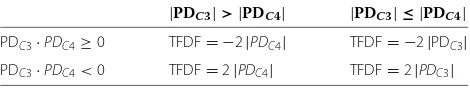
Finally, a TFDF(ωm,τn) is defined as the difference between Fd(ωm,τn)and Fb(ωm,τn)to evaluate the over-all contribution of the data in the time-frequency area (ωm,τn)from electrodes C3 and C4 for two-class
discrim-An ideal time-frequency region for classification should have large discriminative modulations (large Fd(ωm,τn)) and small common modulations (small Fb(ωm,τn)), so the
To examine the behavior of TFDF, we provide its pos-sible values in Table 1 for different cases and present in Figure 2 the ERD/ERS maps and the corresponding TFDF values of 4 Hz, 2-s wide time-frequency regions for an example from a standard dataset. From Table 1, we can see that (1) the values of TFDF are larger for PDC3·PDC4<0 than for PDC3·PDC4≥0, and (2) the values of TFDF are determined by min{|PDC3|,|PDC4|}. Thus, this method tends to seek the time-frequency region where PDC3and PDC4have different signs and large absolute values.
In the ROI, the right hand motor imagery elicits more significant ERD at C3 compared to the left hand motor imagery, which leads to BPLC3(ω∗,τ∗) > BPRC3(ω∗,τ∗), while left hand motor imagery generates more significant ERD at C4 compared to the right hand motor imagery, so we haveBPLC4(ω∗,τ∗) <BPRC4(ω∗,τ∗). Thus,
These different signs of PDC3and PDC4reflect the spa-tial difference of significant ERD between right and left hand motor imageries. On the other hand, large absolute values of PDe represent the large magnitudes of task-related (i.e., right vs. left hand) difference at channel e (i.e., C3, C4), which also contributes to the discrimination between two tasks.
In the literature, a broad frequency band (i.e., 8 to 30 Hz) EEG segments (0.5 to 2.5 s after cue on-set) was typically chosen for feature extraction because it covers theμandβ bands and usually generates good classification results [6]. For this data example, the frequency band (23 to 27 Hz) of the ROI selected by TFDF is in the range ofβband (18 to 25 Hz) but does not completely cover it, and the time segment (1.5 to 3.5 s) is different from the typically used one.
Figure 3A,B shows the distributions of the BP fea-tures extracted from the time-frequency region with the
Table 1 Values of TFDF for different pairs of PDC3and PDC4
|PDC3|>|PDC4| |PDC3|≤|PDC4| PDC3·PDC4≥0 TFDF= −2|PDC4| TFDF= −2|PDC3|
Figure 2ERD/ERS and TFDF values.Maps of ERD/ERS and TFDF values for a subject.(A)ERD/ERS maps of one example: time-frequency selection was performed within the large rectangle (solid line). The small rectangle (dashed line) shows the time-frequency region with the largest TFDF value.(B)TFDF values of the time-frequency regions with 4-Hz wide frequency bands and 2-s wide time segments. The largest value is marked out by a small rectangle.
largest TFDF and of the ones extracted from the rec-ommended broad frequency band EEG segment in a real data example. The linear separation boundary is obtained by Fisher’s LDA in the figure. From the figure, we can see that the BP features extracted from the time-frequency region with the largest TFDF seem more linearly separable than the ones extracted from the rec-ommended broad frequency band EEG segment. The comparison on classification results will be made in the result section to assess the contribution of TFDF to the discrimination between left and right hand motor imageries.
2.2 A criterion based on Fisher’s discriminant
Fisher’s discriminant analysis (Fisher’s LDA) is a very popular classification algorithm in BCI research [19]. It projects high-dimensional data onto a direction and then performs a linear classification in this one-dimensional space. The optimal projection is found by maximizing the separation between two classes. In a one-dimensional fea-ture space, the separation between two classesLandRis defined using the Fisher criterion [20]:
FC= (μ
L−μR)2
(σL)2+(σR)2 (11)
whereμLandμRare the mean values of the feature over all trials for classesLandR, respectively, and (σL)2and (σR)2are the trial-wise variances of the feature.
In feature selection, FC can be used to evaluate the dis-criminative power of each single feature [20]. However, it is not suitable to evaluate the discriminative power of a group of features. Thus, we propose a novel and simplified criterion based on Fisher’s discriminant, calledFscore,Fˆ, and we use it to estimate the discriminative power of a group of features:
wheredenotes the covariance matrix of the feature vec-tor,μdenotes the mean of the feature vector,·2denotes the L2-norm (Euclidean norm), andtr(·) the trace of a matrix.
Without loss of generality, let us discuss this novel cri-terion in a two-dimensional space with the feature vector
f(i)=[f1(i),f2(i)],i=1,. . .,K, whereKis the number of samples (trials) for one class. Thus, the mean of the feature vector for the class isμ =[μ1,μ2], whereμ1andμ2are the mean values off1(i)andf2(i), respectively. We denote byσ12andσ22, the variances off1(i)andf2(i)for the class,
respectively. The trace of the covariance matrix for each class is computed as:
Thus, the trace of the covariance matrix for each class is the mean Euclidean distance between samples to the class center, which reflects intra-class spread.
Compared to FC,Fˆ is a derived version relying on the Euclidean distance between class centers,μL− μR2, to estimate the difference between classes and employing the trace of the covariance matrix to evaluate the variance within a class. Note that this simple expression avoids esti-mating a projection direction as required by the general multi-dimensional expression of Fisher’s discriminant.
In this paper, the BP features [BPC3(i), BPC4(i)] (defined in Equation 3) extracted from the time-frequency ROI are used for classification, so it is also a two-dimensional fea-ture space. We useFˆ to estimate the separation between left hand vs. right hand motor imagery in this feature space: whether(ωm×τn)contains the most discriminative infor-mation. The time-frequency ROI(ω∗,τ∗)is estimated by
the difference between the two sides of brain [7]. In this case, the TFDF value will abnormally increase when using the mean value. As a result, the time-frequency area con-taminated by noise may be selected by error, which may deteriorate classification results when using Fisher’s LDA. On the contrary, for theFscore, outliers will increase the intra-class variance, so they will lower theFscore. Thus, the time-frequency area contaminated by noise will not be selected (due to a lowF score value), though we do not account for the outliers in the calculation of theFscore.
As opposed to the TFDF, theFscore is purely based on statistical characteristics of the features, regardless of neu-rophysiological phenomena linked to a specific task. So, it can be applied in the absence of prior knowledge about task-related neural response.
Figure 4A,B shows theF score and the Euclidean dis-tance between two classes μL− μR2 (which reflects only inter-class difference between two classes) in the time-frequency regions with 4-Hz wide frequency bands and 2-s wide time segments for the data example. The large values of F score mainly appear in the frequency band over 20 Hz for this example, which is quite simi-lar to the distribution of Euclidean distance. However, the maximum value appears in different regions. Figure 3C,D shows the distributions of the BP features extracted from the time-frequency regions with the largestF score, and with the largest Euclidean distance, respectively. The lin-ear separation boundary is also obtained by Fisher’s LDA in the figure. From Figure 3, we can see that the features
extracted from the time-frequency region with the largest F score and the largest Euclidean distance are more lin-early separable than the ones extracted from the broad frequency band EEG segment when using Fisher’s LDA as the classifier. Compared to the features from the time-frequency region with the largest Euclidean distance, the intra-class difference is smaller for the features from the time-frequency region with the largestFscore. As it con-siders the intra-class difference, theFscore is more ade-quate than the Euclidean distance as a two-class separa-tion measurement. The overlap area between two classes is smaller for theFscore than for the TFDF, so that using the features from the time-frequency region selected by F score has less misclassified data (error rate = 11.25% ) than by TFDF (error rate = 13.13%) on the example. This phenomenon indicates that the F score might be more effective than the TFDF. However, the BCI problem is more complicated than a general classification problem [19,20], in particular when training data and testing data are recorded in different sessions [8,25]. Thus, further analysis and comparisons of classification performances with respect to the two criteria on more real data is provided in the ‘Experimental results’ section.
3 Data description and preprocessing
In this study, we used data of the BCI competition IV dataset IIa [26] and IIb [8]. Dataset IIa was recorded in a multi-channel monopolar setting (22 monopolar chan-nels). The parameters of bipolar channels can be adapted
to the experiments. Dataset IIb was recorded over three bipolar channels, C3, Cz, and C4. Details of these two datasets are provided in the following paragraphs.
3.1 Dataset IIa
BCI competition IV dataset IIa [26] contains one training session and one evaluation session of EEG data from nine subjects who performed four classes of cue-driven motor imagery tasks (left hand, right hand, both feet and tongue). Each trial began with a fixation cross and an additional short acoustic warning tone. After 2 s, a cue in the form of an arrow pointing either to the left, right, down, or up (corresponding to left hand, right hand, foot, or tongue) appeared and stayed on the screen for 1.25 s. The subjects were asked to carry out the motor imagery task until 4 s after cue on-set. No feedback was provided.
The EEG signals were recorded by 22 Ag/AgCl elec-trodes (with inter-electrode distances of 3.5 cm) using the left mastoid as reference and the right mastoid as ground (sampling rate 250 Hz). The electrode montage is shown in Figure 5A. For extracting a bipolar channel at the posi-tion of C3 or C4, three different pairs of electrodes can be used, marked asa,p, andlin Figure 5A. Thus, nine possi-ble channel combinations for C3 and C4 are generated for time-frequency optimization.
3.2 Dataset IIb
This dataset consists of two classes (left vs. right hand) cue-driven motor imagery BCI data from nine subjects. The EEG data are recorded in three bipolar channels, i.e., at positions C3, Cz, and C4 (see Figure 5B). The distances between the two bipolar electrodes forming a channel are
pre-determined in this dataset (for details, see [8]). For each subject, five sessions are provided, including three training sessions and two evaluation sessions. The first two training sessions consist of 240 single trials (120 sin-gle trials per session) totally without visual feedback. Each trial started with a fixation cross and an additional short acoustic warning tone. Later, a visual cue was given to guide the subject to execute the corresponding imagina-tion of hand movement over a period of 4 s. The last training session (160 single trials) and both evaluation ses-sions (160 trials per session) were recorded with visual feedback from 0.5 to 4.5 s after the cue on-set (for details, see [8]).
3.3 Experimental goals
The proposed time-frequency optimization methods based on different criteria will first be applied on dataset IIb using only two bipolar channels (C3, C4). The goal of this experiment is to evaluate the effectiveness of the methods in improving the performances of BCI based on few channels only. We first train the methods for each sub-ject on the training data and then evaluate them on the testing data for this subject. Note that training and test-ing sessions are recorded on different days [8,26]. This is called session-to-session transfer [25]. The results of our methods in session-to-session transfers from train-ing sessions to testtrain-ing sessions will be compared with the winners on this dataset in BCI competition IV. Then, we will apply our methods on two bipolar channels (C3, C4) selected from the 22 monopolar channels of dataset IIa. The classification results obtained on dataset IIa will be compared with those obtained by CSP algorithms using 22
monopolar channels to evaluate the interest of the method for electrode reduction.
3.4 Visualization of ERD/ERS maps
The ERD/ERS patterns are usually expressed as percent-age power decrease (ERD) or power increase (ERS) refer-ring to the 1-s interval before the warning tone (for details, see [27]). The time-frequency maps of ERD/ERS for both left (L) and right (R) hands in the bipolar channels C3 and C4 were generated by the Biosig Toolbox using over-lapping 2 Hz bands (step = 1 Hz) in the frequency range between 6 and 32 Hz [28]. The statistical significance of the power increases (ERD) and decreases (ERS) was ver-ified by at-percentile bootstrap test with the confidence interval ofα= 0.05 [27]. Only the significant ERD/ERS are shown in the maps.
3.5 Data preprocessing for time-frequency optimization
Electrooculogram (EOG), originating from ocular activ-ities (e.g., eye movement, blinks), is the most important source of artifacts in BCI. To prevent the influence of EOG artifacts on the classification results, an automated EOG removal method (for details, see [29]) is first applied on the data as required in the BCI competition [30]. Then, for each bipolar channel, 5th order Butterworth filters are applied to compute 19 successive 4-Hz wide frequency bands of signals (F=4 Hz,Fs=1 Hz): 8 to 12, 9 to 13, 10 to 14 Hz,. . ., 26 to 30 Hz, and 15 successive 8-Hz wide fre-quency bands of signals (F=8 Hz,Fs=1 Hz): 8 to 16, 9 to 17, 10 to 18 Hz,. . ., 22 to 30 Hz. Then, 36 overlapping time segments in each frequency band were obtained through 2-, 2.5-, and 3-s wide (i.e.,T=2, 2.5, and 3 s, respectively) sliding windows (12 segments for each sliding window) with 0.2-s step (i.e.Ts = 0.2) moving from 0.5 s after the cue on-set. Those parameters are set based on the expe-rience from competitors reported in BCI competition IV [31] and led to good performances in our previous work [18]. Therefore, there are(19+15)×36= 1, 224 time-frequency areas for subject-specific selection. It has to be mentioned that the selection procedure is not very time-consuming (2 min and 21 s in average, using Matlab 7.10.0 on Window 7 Professional 64bits, CPU 2.66G Hz, RAM 2.0G) and is done offline, so the computational cost is acceptable.
4 Experimental results
In the experiments, the paired samplettest was employed to reveal the statistical significance of the difference between the performances of different methods. The test rejects the null hypothesis at the 0.05 significance level.
4.1 Improving classification performance for dataset IIb
The time-frequency ROI(ωROI ×τROI) of each training dataset is obtained by maximizing the TFDF and the F
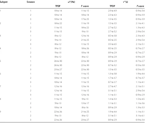
score criteria, respectively. Results are reported in Table 2. These results show that (1) the estimated time-frequency ROIs vary among different subjects, (2) even for the same subject, the estimated ROIs vary among different train-ing sessions, and (3) the two criteria picked out different ROIs for the same training session. The fact that the esti-mation results depend on the subjects is also reflected in the individual differences of timing and frequency of ERD/ERS patterns. Even for the same subject, the tim-ing and frequency of ERD/ERS may shift across sessions [12], which leads to the intra-subject difference in the esti-mation of ROIs between sessions. A typical example of time-frequency maps displaying significant ERD (red) and ERS (blue) in a training session (session 3) for a subject (subject 6) in the dataset is shown in Figure 6. The ROIs estimated by the TFDF are marked out by solid rectangles (10 to 14 Hz, 0.7 to 2.7 s), while the ROIs selected by the F score are displayed as dashed rectangles (11 to 15 Hz, 1.1to 4.1 s). Although the ROIs estimated by the two cri-teria are different, both ROIs contain discriminative ERD patterns between the two classes, indicating that these two criteria could successfully capture the discriminative part of the signal.
To evaluate the contribution of the proposed time-frequency optimization to classification, ten repetitions of cross-validation are performed on each training ses-sion for each subject, using the BP features extracted from the estimated time-frequency ROIs by TFDF andFscore, respectively. In each run, we randomly separated the data into calibration (90%) and test (10%) sets and classified the test data using the Fisher’s LDA obtained from the calibra-tion set. The classificacalibra-tion accuracy (Acc) is defined as the observed agreement between classification outputs and true labels [32]. The cross-validation results are obtained by averaging Acc over 10 runs.
Table 2 Time-frequency ROIs selected by theTFDFandFscore criteria on dataset IIb
Subject Session ω∗(Hz) τ∗(s)
TFDF Fscore TFDF Fscore
1 1 10 to 14 11 to 15 2.9 to 4.9 0.9 to 3.4
2 10 to 14 10 to 14 2.3 to 4.3 0.9 to 3.9
3 10 to 14 17 to 25 1.5 to 3.5 0.9 to 3.9
2 1 18 to 22 11 to 19 1.5 to 3.5 2.1 to 4.1
2 11 to 15 18 to 22 2.7 to 5.2 1.3 to 4.3
3 11 to 15 9 to 13 2.7 to 5.2 2.9 to 5.4
3 1 8 to 12 12 to 16 0.5 to 3.0 2.3 to 4.3
2 9 to 13 21 to 25 0.5 to 2.5 2.9 to 5.4
3 8 to 12 11 to 15 3.5 to 6.5 2.1 to 5.1
4 1 8 to 12 18 to 26 0.5 to 2.5 0.7 to 2.7
2 9 to 13 10 to 18 0.9 to 2.9 0.7 to 2.7
3 8 to 12 8 to 12 0.9 to 2.9 0.9 to 2.9
5 1 26 to 30 22 to 30 0.9 to 2.9 0.7 to 2.7
2 26 to 30 22 to 30 0.7 to 3.2 0.5 to 3.0
3 23 to 27 22 to 30 1.5 to 3.5 0.5 to 3.5
6 1 11 to 15 11 to 15 1.3 to 3.8 1.9 to 4.4
2 10 to 14 11 to 15 1.7 to 3.7 0.7 to 3.7
3 10 to 14 11 to 15 0.7 to 2.7 1.1 to 4.1
7 1 12 to 16 12 to 16 2.7 to 4.7 2.1 to 5.1
2 12 to 16 11 to 15 3.1 to 5.1 2.9 to 5.4
3 11 to 15 12 to 16 1.1 to 3.1 0.9 to 2.9
8 1 11 to 15 9 to 13 1.3 to 3.3 1.5 to 4.5
2 9 to 13 13 to 17 1.1 to 3.1 1.1 to 3.6
3 10 to 14 8 to 16 0.9 to 2.9 1.3 to 3.3
9 1 22 to 26 21 to 25 1.9 to 4.4 1.1 to 3.1
2 9 to 13 8 to 12 3.1 to 5.1 3.1 to 6.1
3 22 to 26 23 to 27 0.9 to 2.9 0.9 to 3.4
To further examine the contributions of these two cri-teria, session-to-session transfers are performed using the training session which has the best classification result in the cross-validation for each subject. As the independent evaluation data are recorded on a different day than the training sessions, EEG signals of the subjects may change significantly from the training data to the evaluation data. This test aims at evaluating the robustness of the methods to non-stationary signals.
In this test, the classifier is parameterized from the selected training session using the BP features from the corresponding(ω∗×τ∗). Theω∗bandpass-filtered EEG segments with the same time length as τ∗ (i.e., T) are obtained from each entire single trial of testing data via a 0.2 s step sliding window to generate continuous clas-sification outputs (see Figure 8). According to the BCI competition requirement, the classification performances
in the session-to-session transfers are measured bykappa coefficient[32]:
κ=(Acc−Pe)/(1−Pe) (18)
wherePeis the chance level for agreement (i.e.Pe = 0.5 for two-class problems, so here κ = 2Acc− 1). Thus, a larger κ value indicates a better classification perfor-mance. The mean kappa value over all subjects of the dataset is denoted byκ¯.
Figure 6ERD/ERS for subject 6.These time-frequency maps display significant ERD (red) and ERS (blue) for subject 6 (a typical example) in BCI competition IV IIb. The areas in the rectangles are the time-frequency ROI selected by the proposed methods based on TFDF (solid line) andFscore (dashed line), respectively.
than FBCSP on this dataset until now [30]. The second place winner employed common spatial subspace decom-position (CSSD) with frequency band and time segment selections [30]. The third place winner applied CSP on spectrally filtered neural time series prediction prepro-cessing (NTSPP) signals [30]. Note that these methods involved frequency and/or time optimization process(es). The results of session-to-session transfers for all meth-ods are provided in Table 4. Theκvalues and the number of electrodes (#E) used in the classification are given. TFDF generates the best meanκvalue (κ¯ = 0.62) among all methods in the independent evaluation. Although the improvements ofκ values yielded by TFDF compared to the first place winner (κ¯ = 0.60,p = 0.12) and the sec-ond place winner (κ¯ =0.58,p=0.18) are not statistically significant due to the limited number of subjects, TFDF outperforms the first place winner for six out of nine sub-jects (except subsub-jects 4, 5, and 8), and the second place winner for six out of nine subjects (except subjects 4, 7, and 9) too. The mean kappa value obtained by theFscore (κ¯ = 0.60) is relatively lower than the one obtained by TFDF (not significantly,p=0.29), but comparable to the first place winner and higher than the second place win-ner (not significantly,p = 0.52). It has to be mentioned that theFscore yields the bestκ values for most subjects (four subjects) among all methods. Further examination of the results show that the poor performance for sub-ject 3 led to a remarkable decrease in mean performance of the F score. In fact, the performances for subject 3
are much poorer than those for the other subjects for all methods, so that results averaged over all subjects might not be representative. Both time-frequency criteria (TFDF andFscore) yield better performances than the third place winner (κ¯ = 0.46, bothp < 0.01) and those obtained by broad band (8 to 30 Hz) EEG segments (0.5 to 2.5 s) with CSP (κ¯ = 0.41, bothp = 0.01) and without CSP (κ¯ =0.53, both not significant byp> 0.05, even if TFDF andF score outperform it for seven and five out of nine subjects, respectively). Thus, both criteria are promising for seeking optimal time-frequency patterns to improve classification performance of BCIs based on a few bipolar channels.
As all of the first three BCI competition winners have used all three bipolar channels (C3, Cz, and C4) pro-vided by the dataset, our methods not only generate good performances but also use less channels, which indicates that they may also be helpful for channel reduc-tion. This potential contribution is validated in the next subsection.
4.2 Electrode reduction for dataset IIa
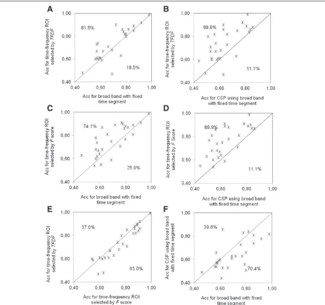
Figure 7Comparison of method performances in the cross-validation on dataset IIb.This figure shows comparisons of method performances in the cross-validation on dataset IIb.(A, B)Scatter plots of classification accuracies (Acc) obtained by using TFDF in time-frequency selection vs. those obtained by broad band (8 to 30 Hz) EEG in a fixed time segment (0.5 to 2.5 s) without and with CSP, respectively.(C, D)Scatter plots of Acc obtained by usingFscore in time-frequency selection vs. those obtained by broad band (8 to 30 Hz) EEG in a fixed time segment (0.5 to 2.5 s) without and with CSP, respectively.(E)Scatter plots of Acc obtained by using TFDF vs. those obtained by usingFscore in time-frequency selection. (F)Scatter plot of Acc obtained by broad band (8 to 30 Hz) EEG in the fixed time segment (0.5 to 2.5 s) with CSP filtering vs. those obtained by the same EEG but without CSP filtering. For the points above the diagonal in each scatter plot, the method iny-axis outperforms the method inx-axis in the cross-validation on the corresponding training session.
in Figure 9. Using theF score generates higher accuracy than using the TFDF for most cases (74.1%).
The optimal channel combinations are selected by com-paring the classification accuracies (choosing the best one) among different combinations in the 10 ×10-fold cross-validation. Optimal channel combinations of C3-C4 and the corresponding estimated time-frequency ROI
for different criteria and different subjects are listed in Table 5.
Figure 8Strategy of session-to-session transfers.This figure shows the strategy of session-to-session transfers for BCI competition IV dataset IIa and IIb. This strategy is the same as what other players used on the same datasets for BCI competition IV [30].
are obtained from each entire single-trial of testing data via a 0.2-s step sliding window to generate continuous classification outputs (see Figure 8).
As this study focuses on the two-class (right vs. left hand) problem, it is difficult to compare with BCI com-petition winners’ results (reported based on a four-class problem including tongue and feet motor imagery data) on this dataset. Here, we compared the results obtained by our method with those obtained by FBCSPa [17], sparse CSP (SCSP) [33], and classic CSP, respectively. Note that FBCSP is believed to be an effective method that well solves the frequency and/or time optimization [14], which has achieved the best classification performance on at least two datasets including dataset IIa in BCI competition IV [30]. SCSP is an optimized CSP that selects the least number of channels in CSP-based classification under a constraint of classification accuracy. SCSP has gener-ated better performances than other channel reduction methods (based on the usual Fisher ratio, mutual infor-mation, SVM, CSP coefficients) and the regularized CSP (RCSP) on BCI competition IV dataset IIa for the right
vs. left hand problem (for details, see [33]). The compar-isons of classification results and the number of electrodes (#E) used in classification between different methods are given in Table 6. As other researchers provided their clas-sification results as clasclas-sification accuracy values (Acc, defined in section ‘Improving classification performance for dataset IIb’) for the right vs. left hand problem on this dataset, we also provide Acc values for the sake of com-parison. Table 6 shows that all methods generate better mean performances than the classical CSP algorithm with all 22 monopolar channels (mean classification accuracy, Acc = 77.26%), indicating the interest of time-frequency selection and electrode reduction. Our method based on Fscore (Acc =79.67%) yields slightly better results than FBCSP (Acc = 79.17%) and SCSP (Acc = 79.07%) but using far less electrodes on this dataset: our method used only the two bipolar channels C3 and C4 (equivalent to four monopolar channels); FBCSP used all 22 monopo-lar channels, and SCSP used 8.55 monopomonopo-lar channels in average [33]. Further examination of individual results shows that our method based onF score generates the
Table 3 Comparison between our method and the first three winners on BCI competition IV dataset IIb
Time-frequency selection Electrodes used Features Classifier
Our method Selected by TFDF orFscore C3, C4 BP LDA
First winner [17] Mutual information-based selec-tion
C3, Cz, C4 FBCSP Naïve Bayes Parzen Window
classifier
Second winner [30] Selected by classification perfor-mance in cross-validation
C3, Cz, C4 CSSD LDA
Third winner [30] Selected by a heuristic search and a selection criterion based on overall classification accuracy in cross-validation.
C3, Cz, C4 CSP Using the best classifier among
Table 4 Performances of different methods in session-to-session transfers on BCI competition IV dataset IIb
κvalues for subjects Mean
#E 1 2 3 4 5 6 7 8 9 κ
TFDF 4 0.44 0.24 0.25 0.93 0.86 0.70 0.55 0.85 0.75 0.62
Fscore 4 0.39 0.25 0.13 0.93 0.88 0.63 0.55 0.88 0.78 0.60
Without CSP 6 0.40 0.24 0.18 0.94 0.39 0.66 0.52 0.81 0.68 0.53
With CSP 6 0.28 0.13 0.11 0.47 0.56 0.13 0.58 0.76 0.67 0.42
FBCSP (first) [17] 6 0.40 0.21 0.22 0.95 0.86 0.61 0.56 0.85 0.74 0.60
CSSD (second) [30] 6 0.43 0.21 0.14 0.94 0.71 0.62 0.61 0.84 0.78 0.58
NTSPP (third) [30] 6 0.19 0.12 0.12 0.77 0.57 0.49 0.38 0.85 0.61 0.46
Best scores are indicated in italics.
best Acc for most subjects (four subjects), indicating that it is the most effective on this dataset. Although the mean classification result of our method based on TFDF (Acc= 78.00%) is slightly lower than those of FBCSP and SCSP, the differences are not statistically significant (p >0.05). Comparing individual performances, our method based on TFDF outperforms FBCSP and SCSP for five out of nine subjects. Moreover, our method based on TFDF also employs less electrodes than FBCSP and SCSP in the classification. Thus, the method based on TFDF still meets the goal of electrode reduction without a significant drop of classification accuracy. Generally speaking, our method based on both criteria can effectively select time-frequency ROI for BCI classification based on only a few channels and therefore contributes to electrode reduction. Let us mention that four electrodes (two bipolar chan-nels) are the smallest set of electrodes required for a good
Figure 9Comparison between performances of TFDF andF score in the cross-validation on dataset IIa.This figure shows the comparison between performances of TFDF andFscore in the cross-validation on dataset IIa.Fscore generated better performance than TFDF in most cases.
performance in left vs. right hand motor imagery discrim-ination on these data. Although using a common reference (e.g., Cz) for C3 and C4 can further reduce the number of electrodes to three, this monopolar setting will signif-icantly deteriorate the classification performances (p < 0.05, see Figure 10). This result, to some extent, also indi-cates that the bipolar setting is more effective than the monopolar setting in a BCI with only few channels.
5 Discussion
A possible widespread use of BCI is limited by many issues, such as the inter-subject variability and the num-ber of electrodes used. Individual differences of brain pattern will deteriorate the performance of BCI when using a general parameter setting, such as features from a broad frequency band (8 to 30 Hz), for all subjects. In this paper, subject-specific time-frequency characteristics are captured by the proposed method to solve this prob-lem, so as to increase the inter-subject robustness. By this subject-specific time-frequency optimization, our method improves the performance of BCI, in particular when only a few channels of data are available. As our method is applied with only two bipolar channels, it also reduces the number of electrodes required in a BCI system.
In the proposed method, two alternative criteria, TFDF andF score, are proposed for measuring the discrimina-tion power of each possible time-frequency region. Both criteria have their novelties and contributions.
Table 5 Optimal channel combinations of C3-C4 and the selected time-frequency ROI on BCI competition IV dataset IIa
Subject C3-C4 ω∗(Hz) τ∗(s)
TFDF F TFDF Fscore TFDF Fscore
1 a-a a-l 12 to 16 11 to 15 1.3 to 3.8 0.5 to 3.0
2 l-l a-l 10 to 14 22 to 26 1.1 to 3.1 0.5 to 3.5
3 a-a a-a 10 to 14 11 to 15 0.7 to 2.7 0.7 to 3.2
4 p-p a-a 21 to 25 11 to 19 0.5 to 2.5 1.1 to 3.1
5 p-l p-a 25 to 29 26 to 30 1.5 to 3.5 1.3 to 4.3
6 l-l l-p 22 to 26 23 to 27 0.5 to 2.5 0.7 to 2.7
7 a-a a-l 19 to 23 18 to 22 0.7 to 2.7 1.1 to 4.1
8 l-l l-p 8 to 12 8 to 12 0.7 to 2.7 0.7 to 3.2
9 a-l p-a 11 to 15 10 to 18 0.5 to 2.5 0.7 to 2.7
for discrimination between foot and right hand motor imagery).
TheFscore is a data-driven criterion and easy to com-pute. As an improvement to the Fisher criterion, which is typically used to measure the discriminative power of a single feature in BCI [20], theFscore provides an effec-tive measure for evaluating the discriminaeffec-tive power of a group of features (a multi-dimensional feature vector), in particular for time-frequency selection in motor imagery-based BCI. As the F score does not require any prior knowledge of neurophysiology, it might be possible to extend its applications on other problems outside the BCI field.
The comparison between the two criteria shows that the F score generated better cross-validation performances than the TFDF on both datasets (see Figures 7E and 9). As theFscore tends to select the time-frequency region by minimizing the overlapping area between two classes (see Figure 3), it is not surprising to have these results when the testing and training data are from the same session and recorded during the same day. However, as we mentioned, a real BCI problem can be more compli-cated than the cross-validation within one session. When the testing and training data are recorded in two sepa-rate days, the unpredictable data evaluation may happen due to slight shift of electrode positions and impedances
and possible changes in the subject’s motivation level [25]. This phenomenon gives TFDF a chance to outper-form theFscore for some subjects (such as subjects 1, 3, and 6 on dataset IIb and subject 4 on dataset IIa), since TFDF selects the time-frequency region not just based on the statistical distribution of features but more on task-relevant ERD, whose frequency characteristics may not change a lot between different days for the same subject.
Although TFDF andFscore alternatively outperformed each other on two different datasets, both of them gen-erated better individual performances than the state-of-the-art methods in most subjects for both datasets as we mentioned in the ‘Experimental results’ session. Thus, generally speaking, our method, either based on TFDF or F score, is robust to session-to-session transfers. As a result, the training data only need to be collected one time for learning the subject-specific time-frequency region and training the classifier, and then the param-eters can be used on the same subject for a long-term on-line classification. The time for collecting the training data, on the one hand, depends on the amount of train-ing data required for well describtrain-ing the different classes; on the other hand, it is affected by the time needed for skin preparation and electrode placing. As the proposed method uses less electrodes than other methods, it will
Table 6 Performances of different methods in session-to-session transfers on BCI competition IV dataset IIa
Acc (%) for subjects Mean
Method #E 1 2 3 4 5 6 7 8 9 Acc
TFDF 4 87.23 66.20 97.81 68.97 64.44 69.44 68.57 96.27 83.08 78.00
Fscore 4 89.36 69.01 97.81 66.38 66.67 72.22 68.57 97.01 90.00 79.67
FBCSPa 22 94.44 52.77 93.05 65.97 88.19 60.41 70.13 94.44 93.05 79.17
SCSP [33] 8.55 91.66 60.41 97.14 70.83 63.19 61.11 78.47 95.13 93.75 79.07
CSP [34] 22 83.51 56.53 97.50 70.00 54.50 62.49 84.50 95.57 90.77 77.26
aThe results of FBCSP on this dataset for right vs. left hand problem are provided by the BCI lab at Institute for Infocomm Research, Singapore, using all 22 monopolar
Figure 10Comparison between using four electrodes and using three electrodes on dataset IIa.This figure shows the comparison between performances of using four electrodes (two bipolar channels) and using three electrodes (two monopolar channels using Cz as common reference) for TFDF andFscore, respectively, in session-to-session transfers on dataset IIa. Reducing the number of electrodes to three significantly deteriorates the classification performance (P<0.05).
save time during skin preparation and electrode placing. The amount of training data required is affected by the dimensionality of features,Df, and the artifacts, since the classifier will fail to give a good performance when the ratio of useful training trials (Numtr) to the dimensional-ity of features, Numtr/Df, is too small [19]. Note that most artifacts in BCI are from EOG, which can be removed by the EOG removal technique, we used in this work to main-tain the amount of useful training trials [29]. Our method reduces the dimensionality of features by using less chan-nels of data, so from this view, it will, to some extent, either improve the classifier training by increasing Numtr/Df or save the time for collecting the training data if keeping the same Numtr/Df as other methods.
Algorithm computational complexity is also an impor-tant factor when considering a real application of BCI. Before further discussion on this issue, we first need to distinguish the computational complexity of off-line anal-ysis and online classification since the importance of these two computational complexities are not at the same level. A time-consuming off-line analysis may not be a real problem for some BCI applications [33], but the speed of online classification does affect the usage of a BCI system. Note that the time-frequency optimization is an off-line analysis; thus, its computational complexity may not be a key issue. Nevertheless, compared to FBCSP [14], this off-line analysis is indeed inexpensive in terms of computational cost in our method, neither involving mutual information calculation nor eigenvalue decompo-sition. In the online classification, band power features are directly extracted from the optimal time-frequency area in our method. This feature extraction step in our method does not involve matrix multiplication, which is needed in CSP-based methods [7]. Furthermore, the computational complexity of the on-line classification is proportional to the dimensionality of feature,Df, when using a classifier like LDA [35]. Our method only uses two channel data,
i.e., Df = 2, which is not larger than any CSP-based methods (Df = 2p, wherepis the number of paired CSP filters). Therefore, thanks to its simplicity, our method is inexpensive in terms of computational complexity for BCI usage.
Last but not least, the proposed method may also con-tribute to reduce the hardware cost in a BCI system since less electrodes are required for a good classification.
6 Conclusions
to address time-frequency optimization for multi-class motor imagery BCIs.
Endnote
aThe results of FBCSP on this dataset for right vs. left
hand problem are provided by the BCI lab at Institute for Infocomm Research, Singapore, using all 22 monopolar channels and the Naïve Bayes Parzen Window classifier.
Competing interests
The authors declare that they have no competing interests.
Authors’ information
Yuan Yang has finished his PhD in Telecom ParisTech and is currently with Delft University of Technology.
Acknowledgements
This work was partially supported by grants from China Scholarship Council and Orange Labs. Authors would like to thank Dr. O. Kyrgyzov (Whist Lab, France) for some useful discussions, Ms. M. Arvaneh and Dr. K. K. Ang (I2R BCI Lab in A*STAR, Singapore) for providing the results of FBCSP and helpful suggestions in experimental comparison.
Author details
1Institut Mines-Telecom, Telecom ParisTech/CNRS LTCI, 46 rue Barrault, Paris 75013, France.2Université de Versailles St-Quentin, Vélizy 78140, France. 3Orange Labs R&D, Issy les Moulineaux 92130, France.4Whist Lab, Paris 75020, France.
Received: 2 October 2013 Accepted: 5 March 2014 Published: 26 March 2014
References
1. JR Wolpaw, N Birbaumer, DJ McFarland, G Pfurtscheller, TM Vaughan, Brain-computer interfaces for communication and control. Clin. Neurophysiol.113(6), 767–791 (2002)
2. N Weiskopf, F Scharnowski, R Veit, R Goebel, N Birbaumer, K Mathiak, Self-regulation of local brain activity using real-time functional magnetic resonance imaging (fMRI). J. Physiol-Paris.98(4–6), 357–373 (2004) 3. R Sitaram, H Zhang, C Guan, M Thulasidas, Y Hoshi, A Ishikawa, K Shimizu,
N Birbaumer, Temporal classification of multichannel near-infrared spectroscopy signals of motor imagery for developing a brain-computer interface. NeuroImage.34(4), 1416–1427 (2007)
4. G Pfurtscheller, FH Lopes da Silva, Event-related EEG/MEG synchronization and desynchronization: basic principles. Clin. Neurophysiol.110(11), 1842–1857 (1999)
5. M Naeem, C Brunner, G Pfurtscheller, Dimensionality reduction and channel selection of motor imagery electroencephalographic data. Comput. Intell. Neurosci.2009, 1–8 (2009)
6. J Müller-Gerking, G Pfurtscheller, H Flyvbjerg, Designing optimal spatial filters for single-trial EEG classification in a movement task. Clin. Neurophysiol.110(5), 787–798 (1999)
7. B Blankertz, R Tomioka, S Lemm, M Kawanabe, KR Müller, Optimizing spatial filters for robust EEG single-trial analysis. IEEE Signal Proc. Mag.25, 41–56 (2008)
8. R Leeb, F Lee, C Keinrath, R Scherer, H Bischof, G Pfurtscheller, Brain–computer communication: motivation, aim, and impact of exploring a virtual apartment. IEEE Trans. Neural Syst. Rehabil. Eng.15(4), 473–482 (2007)
9. B Lou, B Hong, X Gao, S Gao, Bipolar electrode selection for a motor imagery based brain–computer interface. J. Neural Eng.5, 342–349 (2008) 10. JW Osselton, Acquisition of EEG data by bipolar unipolar and average
reference methods: a theoretical comparison. Electroencephalogr. Clin. Neurophysiol.19(5), 527–528 (1965)
11. F Sharbrough, GE Chatrian, RP Lesser, H Lüders, M Nuwer, TW Picton, American electroencephalographic society guidelines for standard electrode position nomenclature. Electroencephalogr. Clin. Neurophysiol.
8, 200–202 (1991)
12. G Pfurtscheller, C Neuper, D Flotzinger, M Pregenzer, EEG-based discrimination between imagination of right and left hand movement. Electroencephalogr. Clin. Neurophysiol.103(6), 642–651 (1997) 13. N Yamawaki, C Wilke, Z Liu, B He, An enhanced time-frequency-spatial
approach for motor imagery classification. IEEE Trans. Neural Syst. Rehabil. Eng.14(2), 250–254 (2006)
14. KK Ang, ZY Chin, H Zhang, C Guan, Mutual information-based selection of optimal spatial-temporal patterns for single-trial EEG-based BCIs. Pattern Recogn.45, 2137–2144 (2011)
15. NF Ince, S Arica, A Tewfik, Classification of single trial motor imagery EEG recordings with subject adapted non-dyadic arbitrary time–frequency tilings. J. Neural Eng.3, 235 (2006)
16. B Wu, F Yang, J Zhang, Y Wang, X Zheng, W Chen, A frequency-temporal-spatial method for motor-related electroencephalography pattern recognition by comprehensive feature optimization. Comput. Biol. Med.
42, 253–263 (2012)
17. KK Ang, ZY Chin, C Wang, C Guan, H Zhang, Filter bank common spatial pattern algorithm on BCI competition IV datasets 2a and 2b. Front. Neurosci.6, 39 (2012)
18. Y Yang, S Chevallier, J Wiart, I Bloch, Time-frequency selection in two bipolar channels for improving the classification of motor imagery EEG, in
34th IEEE Annual International Conference of Engineering in Medicine and Biology Society (EMBC 2012)(IEEE, San Diego, 2012), pp. 2744–2747 19. F Lotte, M Congedo, A Lécuyer, F Lamarche, B Arnaldi, A review of classification algorithms for EEG-based brain–computer interfaces. J. Neural Eng.4, R1–R13 (2007)
20. KR Müller, M Krauledat, G Dornhege, G Curio, B Blankertz, Machine learning techniques for brain-computer interfaces. Biomed. Tech. (Berl).
49, 11–22 (2004)
21. MJ Peters, HJ Wieringa, The influence of the volume conductor on electric source estimation. Brain Topogr.5(4), 337–345 (1993)
22. C Vidaurre, N Kramer, B Blankertz, A Schlögl, Time domain parameters as a feature for EEG-based brain-computer interfaces. Neural Netw.22(9), 1313–1319 (2009)
23. G Pfurtscheller, C Brunner, A Schlögl, FH Lopes da Silva, Mu rhythm (de)synchronization and EEG single-trial classification of different motor imagery tasks. NeuroImage.31, 153–159 (2006)
24. PL Nunez, R Srinivasan, AF Westdorp, RS Wijesinghe, DM Tucker, RB Silberstein, PJ Cadusch, EEG coherency I: statistics, reference electrode, volume conduction, Laplacians, cortical imaging, and interpretation at multiple scales. Electroencephalogr. Clin. Neurophysiol.103(5), 499–515 (1997)
25. B Blankertz, K Müller, D Krusienski, G Schalk, J Wolpaw, A Schlögl, G Pfurtscheller, J Millán, M Schroder, N Birbaumer, The BCI competition III: validating alternative approaches to actual BCI problems. EEE Trans. Neural Syst. Rehabil. Eng.14(2), 153–159 (2006)
26. C Brunner, M Naeem, R Leeb, B Graimann, G Pfurtscheller, Spatial filtering and selection of optimized components in four class motor imagery EEG data using independent components analysis. Pattern Recogn. Lett.
28(8), 957–964 (2007)
27. B Graimann, JE Huggins, SP Levine, G Pfurtscheller, Visualization of significant ERD/ERS patterns in multichannel EEG and ECoG data. Clin. Neurophysiol.113, 43–47 (2002)
28. A Schlögl, C Brunner, BioSig: a free and open source software library for BCI research. Computer.41(10), 44–50 (2008)
29. A Schlögl, C Keinrath, D Zimmermann, R Scherer, R Leeb, G Pfurtscheller, A fully automated correction method of EOG artifacts in EEG recordings. Clin. Neurophysiol.118, 98–104 (2007)
30. M Tangermann, KR Müller, A Aertsen, N Birbaumer, C Braun, C Brunner, R Leeb, C Mehring, KJ Miller, GR Müller-Putz, G Nolte, G Pfurtscheller, H Preissl, G Schalk, A Schlögl, C Vidaurre, S Waldert, B Blankertz, Review of the BCI competition IV. Front. Neurosci.6, 55 (2012)
31. B Blankertz, BCI competition IV: results (2008). http://www.bbci.de/ competition/iv/results/. Accessed 26 September 2011
32. A Schlögl, J Kronegg, JE Huggins, S Mason, G Dornhege, Evaluation criteria for BCI research, inToward Brain-Computer Interfacing(The MIT Press, Cambridge, 2007), pp. 327–342
33. M Arvaneh, C Guan, KK Ang, C Quek, Optimizing the channel selection and classification accuracy in EEG-based BCI. IEEE Trans. Biomed. Eng.
34. Y Yang, S Chevallier, J Wiart, I Bloch, Automatic selection of the number of spatial filters for motor-imagery BCI, in20th European Symposium on Artificial Neural Networks, Computational Intelligence and Machine Learning (ESANN 2012)(ESANN, Bruges, 2012), pp. 109–114
35. D Cai, X He, J Han, Training linear discriminant analysis in linear time, in
IEEE 24th International Conference on Data Engineering (ICDE 2008)(IEEE, Cancun, 2008), pp. 209–217
doi:10.1186/1687-6180-2014-38
Cite this article as: Yang et al.: Time-frequency optimization for discrimination between imagination of right and left hand movements based on two bipolar electroencephalography channels.EURASIP Journal on Advances in Signal Processing20142014:38.
Submit your manuscript to a
journal and benefi t from:
7Convenient online submission
7Rigorous peer review
7Immediate publication on acceptance
7Open access: articles freely available online
7High visibility within the fi eld
7Retaining the copyright to your article
![Figure 1 Positions of C3 and C4. This figure shows positions of C3and C4 (indicated by ellipses) according to the international 10-20system [11].](https://thumb-us.123doks.com/thumbv2/123dok_us/898979.1108355/2.595.57.290.396.691/figure-positions-figure-positions-indicated-ellipses-according-international.webp)