R E S E A R C H
Open Access
An ECSO-based approach for optimizing
degree distribution of short-length LT codes
Peng Luo
1*, Hui Fan
1, Weiguang Shi
2, Xiaoli Qi
2, Yuhao Zhao
1and Xueqing Zhou
1Abstract
Degree distribution plays a great role in the performance of Luby transform codes. Typical degree distributions such as ideal soliton distribution and robust soliton distribution are easy to implement and widely used. Nevertheless, their adaptabilities are not always outstanding in various code lengths, especially in the case of short length. In this paper, our work is to optimize degree distributions for the short-length LT codes by using swarm intelligence algorithm, considering its conceptual simplicity, high efficiency, flexibility, and robustness. An optimization problem model based on sparse degree distributions is proposed in the first place. Then, a solution on the basis of an enhanced chicken swarm optimization algorithm, termed as ECSO, is designed for the problem. In ECSO, substitution of bottom individuals, revision of chicks’ update equation, and introduction of differential evolution are designed to enhance the ability of optimization. Simulation comparisons show that the proposed solution achieves much better performance than two other swarm intelligence-based solutions.
Keywords:Fountain codes, LT code, Degree distribution, Differential evolution, Chicken swarm optimization
1 Introduction
Power line communication (PLC) is regarded as a ser-ious candidate for the realization of smart grid networks due to its high data rate, easy connection between de-vices, broad coverage, and low-cost deployment. For PLC, data transmission over long distances and at high frequencies is a challenging issue, and some schemes have been proposed on the basis of cooperative ap-proaches. Among them, the cooperative communication schemes leveraging digital fountain code (DFC) attract considerable attention from researchers because of their lower redundancy and higher reliability [1,2].
Developed by Byers et al. in 1998, DFC is a popular probabilistic forward error correction scheme [3]. One of the most distinctive properties of DFC is rateless. Encoded packets are continuously delivered like a fountain, and any receiver can reconstruct the source data once a sufficient number of packets are received [4]. Examples of fountain codes include LT codes [5], raptor codes [6], and online codes [7]. Compared with the two others, LT codes have simpler encoding procedure and are more representative,
leading a wider scope of application, including deep space communication [8], data distribution [9], wireless sensor networks [10], and cloud storage [11].
A good degree distribution is necessary for the above-mentioned DFC-based cooperative communication schemes, since degree distribution plays a crucial role in the performance of encoding and decoding of LT codes. The encoder generates an encoded symbol on the basis of a particular probability distribution, the so-called degree distribution, and the decoder utilizes the same degree distribution to recover the original input symbol. There are five suggested degree distributions: (1) all-at-once distribution; (2) binomial distribution (BD); (3) binomial exponential distribution (BED); (4) ideal soliton distribution (ISD); and (5) robust soliton distribution (RSD). Although the distributions men-tioned above are easy to be implemented, their per-formance varies in distinct occasions. Correspondingly, a large amount of attention has been paid to improve the performance of LT codes by optimizing the degree distribution, some achievements have been made also.
* Correspondence:[email protected]
1State Grid Hebei Electric Power Research Institute, Shijiazhuang 050021, China
Full list of author information is available at the end of the article
According to the length of the LT codes, existing methods for optimizing degree distribution can be di-vided into two categories: the methods for long length (MLL) [12–15] and the methods for short length (MSL) [16–19]. In this paper, our work is seeking a simple MSL; hence, a review of MLL is briefed. Among MSL, in [16], the decoding process was studied as a Markov chain and an analytical combinatorial approach is pre-sented. In [17], the effect of the RSD on decoding delay as well as percentage overhead for LT codes with small message size was investigated. Results showed that the decoding latency can be decreased by optimizing the RSD’s parameters. In [18], Esa Hyytiä et al. proposed an iterative optimization algorithm, whose idea was bor-rowed from importance sampling theory. In [19], the de-gree optimization problem was reformulated in form of standard semidefinite programming (SDP) on AND–OR tree analysis of BP algorithm. Considering a large num-ber of optimization variables in the obtained SDP, the authors proposed an alternative linear program that can be solved numerically for a reasonable number of source packets. It is noteworthy that the attempts above were met with limited success. For example, the approach in [16] is effective only when the message length is less than 30. For the approach in [17], it relies heavily on heuristic knowledge from simulation test and it lack of targeted strategy. Importance sampling theory utilized in [18] still needs further exploration for better performance. Accord-ingly, investigating MSL remains an open problem.
During the past few decades, natured-inspired computa-tion algorithms have attracted significant attencomputa-tion from scholars as an attractive issue. Among them, the most suc-cessful are evolutionary computation (EC) and swarm intelligence (SI). EC algorithms are search methods that take their inspiration from natural selection and survival of the fittest in the biological world. SI algorithms are in-spired by the collective behavior of social systems (such as fish schools, bird flocks, and ant colonies) and have be-come an innovative computational way to solving hard optimization problems. Due to the simplicity and flexibil-ity of EC and SI, some schemes have been developed for the degree distribution optimization of short-length LT codes [20–22]. Among them, the solution in [22] is a typ-ical SI-based instance, in which Deng et al. utilized a par-ticle swarm optimization (PSO) algorithm with a gradient to design the degree distribution for reducing the decod-ing overhead. The evaluation upon sparse degree distribu-tions has approved the effectiveness to some extent. However, this SI-based optimization can easily to fall into the local solution because of the inherent characteristics of the PSO.
Recently, chicken swarm optimization (CSO), a novel SI algorithm mimicking hierarchal order and behaviors of the chicken swarm, has been proposed in [23]. In
CSO, the individuals follow diverse approaches of evolu-tionary according to their fitness values, which is lacking in most of typical EC and SI algorithms such as genetic algorithms (GA), differential evolution (DE), and PSO. Statistical comparisons on 12 benchmark problems illus-trate its superiority in the terms of accuracy, efficiency, and robustness. Many endeavors have also been made to further improve the performance of CSO [24–26]. In [24], for optimally selecting the sensor nodes to form a virtual node antenna array, a novel swarm intelligence optimization algorithm called cuckoo search chicken swarm optimization (CSCSO) is proposed, in which chaos theory, inertia weight Lévy flight, and grade mech-anism are leveraged to improve the performance. For the problem that the typical chicken swarm optimization can easily fall into a local optimum in solving high-dimensional problems, an improved chicken swarm optimization is proposed in [25]. The relevant parameter analysis and the verification of the optimization capabil-ity by test functions in high-dimensional case were made. In [26], MPCSO, an enhanced version incorpo-rated with monomers turbulence in rooster (MTR) strat-egy and particle renovation in hen (PRH) stratstrat-egy, is proposed for solving L-RNP problem. Simulation results prove the effectiveness of these improved algorithms. Specifically, it is recognized that CSO offers an effective approach to the optimization of complex problems.
Motivated by the above facts, our work in this paper is to optimize the degree distribution for short-length LT codes by leveraging CSO. Firstly, we provide a framework for the optimization problem, where the form with sparse degree distributions is considered. The optimization ob-jective is to minimize decoding overhead with recov-ering the entire original data. Secondly, a solution based on an enhanced CSO algorithm is put forward for achieving optimal degree distributions. Substitu-tion of bottom individuals is drawn to enhance the efficiency of roosters’ cruising. The update equation of chicks is also revised. Besides, DE strategy is intro-duced to refine the information interaction among the individuals. Finally, we design and carry out simu-lation experiments. Simusimu-lation results show that the addressed approach is capable of achieving much bet-ter performance than other algorithms. To the best of our knowledge, this is the first work that optimizes the degree distributions of LT codes by utilizing CSO-based algorithm.
2 LT coding method
2.1 Encoding and decoding of LT codes
Three procedures consist the encoding process of LT codes. Firstly, the source data is partitioned intokinput symbols. Secondly, a degree d is chosen randomly ac-cording to an adopted degree distribution ρ(d) to gener-ate an encoded symbol, with 1≤d≤dmax, dmax is the
maximal degree value, Pdmax
d¼1ρðdÞ ¼1. The degreed
de-cides the number of input symbols combined into an encoded symbol. Thirdly, d input symbols, also named neighbors, are chosen randomly and accumulated via XOR operation to produce an encoded symbol at the LT encoder. The last two procedures work periodically to generate a number of encoded symbols.
At the LT decoder, belief-propagation (BP) algorithm is utilized in common to reconstruct source data from then encoded symbols. Usually, n is slightly bigger than k. Firstly, the decoder searches the encoded symbols with only one (degree-1) neighbor to decode directly. Secondly, the recovered input symbols are exclusive-XORed with their neighbors to update the encoded symbols. Mean-while, the edge between each encoded symbol and its neighbor is removed. These two procedures will be iter-ated until no encoded symbol with degree-1 is available.
2.2 Degree distribution
The behavior of LT code is mainly determined by the de-gree distribution and the number of encoded symbols received by the LT decoder. The overhead ε=n/k indi-cates the performance of LT code and depends on a given degree distribution. In [5], Luby designed an ISD based on an analogy of throwing an infinite number of balls randomly intoknumber of bins:
ρð Þ ¼d
In the ideal case, the overhead equals to 1, indicating the best performance. However, ISD works poorly in practice, since the decoding behavior of finite length LT codes may fluctuate among randomly encoded symbol. Hence, in the same paper, Luby addressed another de-gree distribution, known as RSDμ(d). By adding an ad-justment termτ(d) toρ(d),μ(d) can be expressed as is the probability of decoding failure. Further discussion and reasoning for this distribution can be found in the references [6].
Compared with ISD, RSD is more viable and practical. The performance analysis of RSD is derived based on the assumption that k is infinite. However, source data in practice is usually divided into finite pieces, and as a re-sult, the feature of LT code under RSD will not exactly match the mathematical analysis, especially in the case of smallk.RSD provides an easy way to construct a distribu-tion that works well but not optimally. In this paper, we will propose a more universal and effective approach for optimizing degree distribution of LT codes with short length, by leveraging an emerging SI algorithm.
3 Optimization problem
3.1 Variables design based on sparse degree distribution For the SI-based optimization, the challenge of huge searching space is a pivotal issue. When the degrees ran-ging from 1 to k are planned to be optimized, the di-mension of searching space equals to the source data length k. In this situation, due to the complexity of en-coding and deen-coding of LT codes, it is not easy for the SI-based algorithm to achieve a desirable solution within an acceptable time, especially in the case of data length reaching hundreds, thousands, or more.
To reduce the search space dimension, sparse degree distribution (SDD) is chosen in our work for designing the variables that can properly stand for the probability mass function ρ(d). In SDD, partial degrees are consid-ered to have zero probabilities, which simplify the design of the degree. Adopting a SDD has been an alternative scheme used in LT codes optimization [2, 18,20–22]. In particular, we consider distribution where positive prob-abilities are assigned to optimization components whose indices are powers of two and less thank, i.e., fordj= 2j and j= 1, 2, …, D. dmax= 2D is the highest indice
with dmax<k. On the other hand, all the other degrees
are assumed to have zero probabilities. Accordingly, the variables to be designed can be expressed as vectors Ω = {ρ(d1), ρ(d2), …, ρ(dD)}.Obviously, the dimension of
search space isDand much less than the typical valuek.
3.2 Objective formulation
efficiency is indicated by the decoding overhead, related to the average number of encoded symbols required for successfully recovering all original data. A smaller aver-age decoding overhead signifies a higher efficiency. On the other hand, complexity is generally evaluated by the average degree of encoded symbols required for success-fully recovering all original data. It is also hoped that the average degree is as small as possible.
In this paper, we choose efficiency to formulate the ob-jective function. Suppose the encoded symbols transmit in an ideal channel and T denotes the number of encoded symbols required for decoding an input symbol. Then, our optimization objective can be formulated as
overhead¼E T½ −k
k ; ð4Þ
whereEis the expectation of received encoded symbols’ number.
During the iteration, for simplifying the calculation, we directly employ the mean of T to measure the per-formance of degree distribution instead of theoverhead. Correspondingly, the fitness function can be defined as
fð Þ ¼Ω 1 m
Xm
r¼1T rð Þ; ð5Þ
wheremis the number of decoding trials.T(r) is the num-ber of encoded symbols required for a successful decoding in therth sample. Accordingly, the design of degree distri-bution can be denoted as a minimization problem
OSð Þ ¼Ω arg minð ð Þf Þ: ð6Þ
To accurately evaluate the value of T, a stepwise de-coding mode is employed and works as follows.
Step 1: When the number of encoded symbols at the decoder is bigger than⌈k(1 +δ)⌉, the BP decoding starts to work. δ is a default value of overhead set by the de-signer.⌈⌉denotes floor rounding calculation.
Step 2: If the decoder fails to decode the whole input symbols, it recruits another ⌈kδ⌉-encoded symbols and continues the decoding operation.
Step 3: If the decoder succeeds in decoding the whole input symbols, the amount of encoded symbols is re-corded and the stepwise decoding mode is terminated. If not, go back to Step 2.
4 ECSO-based solution
4.1 Preliminaries of typical CSO
Proposed by X.B. Meng et al., chicken swarm optimization is a bio-inspired metaheuristic optimization algorithm that mimics a hierarchal order in chicken swarm and behaviors of the chicken swarm [23]. The rules of chicken behavior in CSO can be summarized as follows:
4.1.1 Division and classification
The entire chicken swarm is divided into several groups, and each group consists of a rooster, some hens, and several chicks. Each type of chickens follows specific laws of motions.
4.1.2 Hierarchy and relationship
The fitness value of the chickens outlines a hierarchy of the swarm. The individuals with the best fitness are regarded as the roosters, each of which is a leader of the group. The individuals with the worst fitness values are considered as chicks. The others would be the hens. The hens randomly choose which group to live in. The mother-child relation-ship between the hens and the chicks is also randomly established. The swarm hierarchy, dominance relationship, and mother-child relationship in a group will remain un-changed until an update command is issued. In the typical CSO, the update command arrives everyGtimes.
During the evolutionary, each individual follows their group-mated rooster and keeps moving to find a better position, whereas the different type of chickens employ different movement pattern. Suppose N stands for the number of original chickens in the swarm. NR, NH, NC, and NM respectively represent the number of roosters, hens, chicks, and mother hens. N=NR+NH+NC. As-sume all the virtual chickens, depicted by their positions xi,j(t) at stept, search for food in aD-dimensional space where i∈[1, …,N], j∈[1, …,D], and t∈[1, …,W]. W is the iteration number. The roosters with better fitness values can search for food in a wider range of places than those roosters with worse fitness values, and their movements can be formulated as
xi;jðtþ1Þ ¼xi;jð Þt 1þRandn 0; σ2
where Randn(0, σ2) indicates a Gaussian distribution with mean 0 and standard deviationσ. ε is the smallest constant utilized to avoid zero-division error.fiexpresses
the fitness value of the rooster xi. w is the index of a
rooster chosen randomly from rooster’s group.
Hens follow their group-mated roosters to search for food. More dominant hens would have an advantage in competing for food than more submissive ones. These phenomena can be formulated mathematically as
c2¼ exp fr2−fi
; ð11Þ
where Rand is a uniform random number limited in [1, 0]. r1indicates a rooster’s index, which is theith hen’s
group-mate, and r2 (r1≠r2) indicates the index of the chicken
(rooster or hen) selected randomly from the swarm. The chicks move around with their mother to search for food. This is formulated below.
xi;j ðtþ1Þ ¼xi;j ð Þ þt FL xm;jð Þt − xi;j ð Þt
;
ð12Þ
wherexm,j (t) is the position ofith chick’s mother.FLis a coefficient in the range [0, 2], representing the ability of the chick for following its mother to seek food.
4.2 Enhanced CSO algorithm
In this section, an enhanced CSO algorithm for designing degree distribution of short-length LT codes is proposed and described. For ease of description and comparison, we termed the proposed algorithm as ECSO. Fundamentally, the enhancement in ECSO comprises three parts: substi-tution of bottom individuals (SBI), revision of chicks’ up-date equation (RCE), and introduction of DE (IDE). For a better understanding, the principles of these three strat-egies are illustrated as follows.
4.2.1 Substitution of bottom individuals
Among a large chicken swarm, the individuals with worst fitness values, a certain part of chicks, basically fail to not only have a beneficial impact on the evolution process due to their poor performance, but also cause a waste of calculation amount. Recognizing this fact, in our work, the NW individuals with the worst fitness value are defined as bottom individuals and expected to be eliminated. On the contrary, roosters’positions report the best behaviors of the whole swarm and predetermine the rapidity and accuracy of convergence. The perturb-ation number of each rooster during a single evaluperturb-ation plays a major role in the efficiency of the rooster swarm. A larger perturbation number implies a higher chance of improvement of the rooster search.
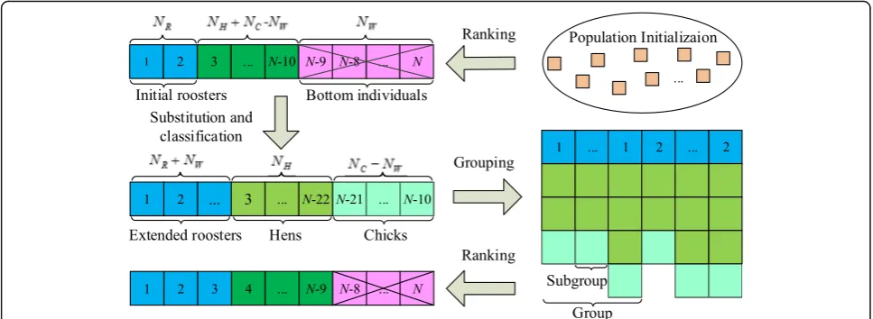
Based on the two points above, SBI strategy shown in Fig.1is suggested as follows. Firstly, each bottom individ-ual is substituted by a rooster to leave the size of popula-tion unchanged and facilitate the design of the optimization process. Treating NR as the initial size of roosters, the extended size of roosters will reachNR+NW after the substitution operation. For ease of programming, letNWbe an integer multiple ofNR. Secondly, according to the diversity of the individuals’ status, the extended rooster swarm is classified intoNRgroups, each of which contains roosters with the same fitness value. In the typ-ical CSO algorithm, the hens randomly choose which
group to live in so as to increase the variety of the evolution. Whereas in our approach, hens are allocated to the group where roosters provide the nearest neighbor Euclidean distance to enhance the convergence of great population. The chicks join in the group where their mother lives in. Afterward, each group is divided intoNW/ NR+ 1 subgroups, each of which consists of one rooster, several hens, and a few chicks. The allocation of chicken is generated randomly. Thirdly, in order to balance the rela-tionship between the convergence and variety, the initial size of the rooster is suggested to increase by degrees dur-ing the iterative evolution. For instance,NRequals to 2 in the former half iteration of the evolution process while in-creases to 3 in the latter half iteration.
4.2.2 Revision of chicks’update equation
In typical CSO, each chick only achieves position infor-mation from their own mother, rather than the roosters. In this case, it is hard for the chicks to obtain a better solution once their mothers fall into local optimum. Hence, the update equation of the chick is modified, and the formula (12) is rewritten as
xi;jðtþ1Þ ¼xi;jð Þ þt FL xm;jð Þt −xi;jð Þt
þc3 xrbest;jð Þt −xi;jð Þt
; ð13Þ
wherec3indicates the learning coefficient.rbestexpresses the index of the rooster with the best fitness value in the current iteration.
4.2.3 Introduction of DE
It should be noted that, in CSO, the information inter-action among the individuals mainly occurs within a limited range, weakening the global optimization ability and deep optimization ability. For the roosters, the per-turbation range is decided by σ only and the states of hens and chicks are not fully utilized. Besides, it would be hard to obtain a better performance by simultan-eously updating the individuals’states on all dimensions, because of their own superior fitness values. That is to say, the improvement upon a certain dimension would be possibly counteracted by the deterioration of some other dimensions. As for the update of hens, as shown in (8), a hen can only follow roosters to search for food, but fail to share information with other hens. It is necessary and possible to further improve the performance of the CSO by refining the manner of information interaction.
selection are operated for the new generation. DE/rand/ 1/bin in [28] is chosen as the scheme of DE strategy.
4.3 Procedure of ECSO-based approach
Overall, the procedures of the ECSO-based approach for optimizing degree distribution of short-length LT codes are suggested as below:
Step 1: Initialize a starting distributionΩI= [pI, 1, pI, 2, …, pI,j, …, pI,D] in terms of the input
symbolskand the number of probability degree distributionsN, withpI,j∈(0, 1) and
PD
j¼1pI;j
¼1.
Step 2: Utilize the starting distributions to construct the initial populations of ECSO algorithm. Each probability degree distribution stands for the position of a chicken in the swarm, and there are totallyNchickens. The position of theith individual in the initial solution is expressed asxIi
¼ ½pI
i;1; pIi;2;…; pIi;j; …; pIi;D.
Step 3: Start the optimization process witht= 1 and calculate the fitness values through formula (4). Step 4: Ift%G= 1, establish hierarchal order and
execute SBI operation based on the sorted fitness values. Update the position of roosters, hens, and chicks by using formula (6), formula (8), and formula (13) respectively. Normalization is also leveraged to ensurePDj¼1pi;jðtÞ ¼1. [pi, 1(t),pi, 2(t), …,pi,j(t),…,pi,D(t)] denotes the state of the
ith individual in thetth iteration.
Step 5: Start the mutation operation as the first process of DE strategy. Three individuals are chosen randomly for generating a mutant vector given by
viðtþ1Þ ¼xy1ðtþ1Þ þM xy2ðtþ1Þ−xy3ðtþ1Þ
; i≠y1≠y2≠y3;
ð14Þ
where M∈[0, 2] denotes the amplification factor.y1,
y2, y3∈[1, …,N] denotes random indexes, respectively.
Step 6: Execute the binomial crossover operation as the second process of DE strategy. Use the mutant vectors and positions of individuals to obtain corresponding trial vectors. The rule is presented as
ui;jðtþ1Þ ¼ vi;j tþ 1
ð Þ for Randð Þ≤j CR or j¼jrand xi;jðtþ1Þ for Randð Þ≥j CR and j≠jrand
;
ð15Þ
where Rand(j) is the jth evaluation of a uniform random number generator with the outcome ∈[0, 1]. CR∈[0, 1] represents crossover probability. jrand is selected ran-domly from 1 toD.
Step 7: Switch to the selection operation as the third process of DE strategy. Use the greedy criterion to decide whether a trial vector would become a member of the next generation. The greedy criterion is provided as
xiðtþ1Þ ¼uiðtþ1Þ for f uð iðtþ1ÞÞ<f xð iðtþ1ÞÞ: ð16Þ
Step 8: Sett=t+ 1, if the step meets the maximum iteration, terminate the algorithm and output the optimal solution; otherwise, go to Step 4.
Fig. 1 Framework of SIB strategy. Describes the mechanism and process of the substitution of bottom individual (SBI) strategy. After the
5 Simulation results
5.1 Simulations setup
In this section, simulation experiments have been imple-mented using MatLab R2014a platform. Two simulation jobs are carried out to evaluate the performance of the proposed approach. Firstly, we investigate the effective-ness of SBI, RCE, and IDE and evaluate the performance of the ECSO algorithm in comparison with other algo-rithms by using 12 benchmark functions presented in Table 1. Secondly, for validating the effectiveness of the ECSO-based approach, three instances, namely K32, K64, K128, are provided to illustrate the optimization capability under different short-length scenarios, among whichkis set as 32, 64, and 128. Correspondingly,Dis set as 5, 6, and 7, respectively. It is clear that the bigger thekis, the harder the design of degree distribution becomes.
5.2 Testing on the benchmark functions
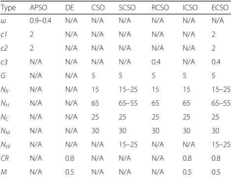
To validate the effectiveness of SBI, RCE, and IDE, we termed the algorithm combining SBI and CSO as SCSO, the algorithm combining RCE and CSO as RCSO, and the algorithm combining IDE and CSO as ICSO. Three algorithms Adaptive PSO (APSO) [29], DE [28], and CSO [23] are chosen and compared in this section. Among them, APSO has a linear de-creasing inertia weight when the number of iterations increases. DE simulates genetic processes (mutation, crossover, and selection operations) to generate the optimal solution by iterations. For all the algorithms, the population size is set as 100; the maximum num-ber of generations is 100. The dimension of searing space is 10. The basic control parameters of the seven algorithms are given in Table 2. Note that, for SCSO algorithm and ECSO algorithm, set NR=NW=15, NH=65 during the former half iteration of the evolu-tion process and set NR=NW=25, NR=55 during the latter half iteration of the evolution process.
According to the principle of Monte Carlo, all the al-gorithms are executed 40 times independently to achieve statistical results.
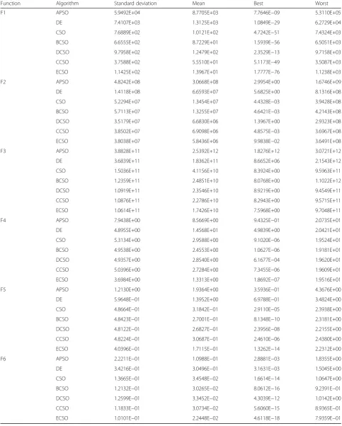
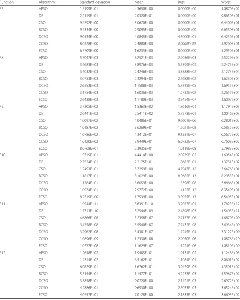
Tables 3 and 4 show the statistical results obtained from the 40 runs, under the benchmark functions. The mean results, the best results, the worst results, and the standard deviation of fitness value are reported. Itali-cized data in the table indicate the best values among those achieved by all three algorithms. It is obvious that SBI strategy, RCE strategy, and IDE strategy could greatly improve the performance of the CSO, for most of the benchmark functions tested. Besides, the three strategies could work harmoniously since ECSO that combines all the three strategies almost invariably ob-tains the smallest values compared to the others. Take F12 for instance, the mean final fitness values of SCSO, RCSO, and ICSO are 11.477, 9.072, and 9.693, respect-ively, and the corresponding values of APSO, DE, and CSO are 19.405, 65.162, and 16.762, respectively, whereas ECSO wins the best value, 7.073.
5.3 Comparison and analysis on the degree distribution optimization
To evaluate the performance of the ECSO-based ap-proach, PSO-G-based approach in [19] and typical CSO-based approach are compared in this section. Just like the above section, all three algorithms are executed 40 times. For all the algorithms, the size of the popula-tion is set as 100 and the maximum number of genera-tions is set as 80. For PSO-G-based approach, the parameters are the same to those in [22]. For CSO-based approach and ECSO-based approach, the pa-rameters are the same to those in Table 2. The rest of the parameters are set as follows:δ= 0.05 andm= 20.
Statistical results for instances K32, K64, and K128 are shown in Tables5, 6, and7. For one thing, it is obvious Table 1Benchmark functions tested in this paper
Function ID Bounds Optimum
High conditioned elliptic F1 [−100,100] 0
Penalized F2 [−50,50] 0
Rosenbrock F3 [−30,30] 0
Ackley F4 [−32,32] 0
Griewank F5 [−600,600] 0
Sphere F6 [−100,100] 0
Step F7 [−100,100] 0
Schwefel’s P1.2 F8 [−100,100] 0
Rastrigin F9 [−5.12,5.12] 0
Axis parallel hyer-ellipsoid F10 [−5.12,5.12] 0
Schwefel’s P2.22 F11 [−100,100] 0
Quartic F12 [−1.28,1.28] 0
Table 2Parameter settings for the seven algorithms
Type APSO DE CSO SCSO RCSO ICSO ECSO ω 0.9–0.4 N/A N/A N/A N/A N/A N/A
c1 2 N/A N/A N/A N/A N/A 2
c2 2 N/A N/A N/A N/A N/A 2
c3 N/A N/A N/A N/A 0.4 N/A 0.4
G N/A N/A 5 5 5 5 5
NR N/A N/A 15 15–25 15 15 15–25
NH N/A N/A 65 65–55 65 65 65–55
NC N/A N/A 25 25 25 25 25
NM N/A N/A 30 30 30 30 30
NW N/A N/A N/A 15–25 N/A N/A 15–25
CR N/A 0.8 N/A N/A N/A 0.8 0.8
M N/A 0.5 N/A N/A N/A 0.5 0.5
Table 3Performance comparison of all algorithms based on benchmark functions F1–F6
Function Algorithm Standard deviation Mean Best Worst
F1 APSO 5.9492E+04 8.7705E+03 7.7646E−09 5.3110E+05
DE 7.4107E+03 1.3125E+03 1.0849E−29 6.2729E+04
CSO 7.6889E+02 1.0121E+02 4.7242E−51 7.4324E+03
BCSO 6.6555E+02 8.7229E+01 1.5939E−56 6.5051E+03
DCSO 9.7958E+02 1.2479E+02 2.3529E−13 9.7158E+03
CCSO 3.7588E+02 5.5510E+01 5.1173E−49 3.5087E+03
ECSO 1.1425E+02 1.3967E+01 1.7777E−76 1.1238E+03
F2 APSO 4.8242E+08 3.0668E+08 2.9954E+00 1.6746E+09
DE 1.4118E+08 6.6593E+07 5.6825E+00 8.1316E+08
CSO 5.2294E+07 1.3454E+07 4.4328E−03 3.9428E+08
BCSO 5.7113E+07 1.3255E+07 4.6421E−03 4.2143E+08
DCSO 3.5179E+07 6.6830E+06 1.3967E+00 2.9323E+08
CCSO 3.8502E+07 6.9098E+06 4.8575E−03 3.6967E+08
ECSO 3.8038E+07 5.8436E+06 9.9838E−02 3.6491E+08
F3 APSO 3.8828E+11 2.5392E+12 1.8276E+12 3.0721E+12
DE 3.6839E+11 1.8362E+11 8.6652E+06 2.1543E+12
CSO 1.5036E+11 4.1156E+10 8.3924E+00 9.5963E+11
BCSO 1.2359E+11 2.4851E+10 8.0768E+00 1.1022E+12
DCSO 1.0919E+11 2.3546E+10 8.9219E+00 9.4549E+11
CCSO 1.0876E+11 2.2786E+10 8.2943E+00 9.5715E+11
ECSO 1.0614E+11 1.7426E+10 7.5968E+00 9.7048E+11
F4 APSO 7.9438E+00 8.5669E+00 9.4325E−01 2.0735E+01
DE 4.8955E+00 1.4568E+01 4.9839E+00 2.0421E+01
CSO 5.3134E+00 2.9588E+00 9.1020E−06 1.9524E+01
BCSO 4.9538E+00 2.4553E+00 1.0627E−06 1.9181E+01
DCSO 4.9357E+00 2.8540E+00 6.1677E−04 1.9620E+01
CCSO 5.0396E+00 2.7284E+00 7.3455E−06 1.9609E+01
ECSO 3.6984E+00 1.3313E+00 1.8692E−07 1.9516E+01
F5 APSO 1.2130E+00 1.9364E+00 3.5936E−01 4.3676E+00
DE 5.9648E−01 1.3952E+00 6.9788E−01 3.4824E+00
CSO 4.8664E−01 3.1842E−01 2.9110E−05 2.3938E+00
BCSO 4.8423E−01 2.7001E−01 8.1348E−10 2.3181E+00
DCSO 4.8122E−01 2.6827E−01 2.3956E−08 2.2155E+00
CCSO 4.8224E−01 3.0687E−01 2.4610E−06 2.4380E+00
ECSO 4.0396E−01 1.7115E−01 1.3262E−14 2.2312E+00
F6 APSO 2.2211E−01 1.0988E−01 2.8881E−03 1.8355E+00
DE 3.4216E−01 3.0496E−01 3.1631E−03 1.5045E+00
CSO 1.3665E−01 3.4548E−02 1.6614E−14 1.0647E+00
BCSO 1.2132E−01 3.0265E−02 8.0612E−16 9.2391E−01
DCSO 1.2599E−01 3.3452E−02 4.3039E−12 1.0142E+00
CCSO 1.1833E−01 3.0734E−02 5.6060E−15 8.9365E−01
Table 4Performance comparison of all algorithms based on benchmark functions F7–F12
Function Algorithm Standard deviation Mean Best Worst
F7 APSO 1.7199E+01 4.3650E+00 0.0000E+00 1.0870E+02
DE 2.2119E+01 2.0320E+01 0.0000E+00 9.8650E+01
CSO 9.4792E+00 3.0670E+00 0.0000E+00 6.4400E+01
BCSO 9.4334E+00 2.9095E+00 0.0000E+00 6.6550E+01
DCSO 9.0134E+00 4.0845E+00 4.5000E−01 6.4250E+01
CCSO 8.0428E+00 2.4880E+00 0.0000E+00 5.9200E+01
ECSO 6.7709E+00 1.6255E+00 0.0000E+00 5.2950E+01
F8 APSO 5.7047E+03 8.2521E+03 2.2036E+03 2.5229E+04
DE 3.4683E+03 3.8976E+03 5.5399E+02 2.2475E+04
CSO 3.4032E+03 2.4246E+03 3.3888E+02 2.1273E+04
BCSO 3.0753E+03 2.3294E+03 2.7688E+02 1.6230E+04
DCSO 2.6553E+03 1.1508E+03 5.3335E−05 1.6955E+04
CCSO 3.1754E+03 1.6036E+03 1.2732E+02 2.2657E+04
ECSO 2.6438E+03 1.1180E+03 3.9454E−07 1.6007E+04
F9 APSO 2.7305E+02 1.5363E+02 1.8616E+01 1.1794E+03
DE 2.0441E+02 2.5411E+02 5.7273E+01 1.0046E+03
CSO 1.0097E+02 4.0486E+01 9.6601E−06 6.2801E+02
BCSO 1.0187E+02 3.6269E+01 1.2021E−08 6.5835E+02
DCSO 1.0786E+02 4.3412E+01 9.1331E−07 6.5675E+02
CCSO 1.0120E+02 3.9449E+01 6.0732E−07 6.7608E+02
ECSO 8.0768E+01 2.3935E+01 1.0119E−08 5.7983E+02
F10 APSO 1.9719E+01 4.4414E+00 2.0279E−02 1.6054E+02
DE 2.7524E+01 2.2175E+01 1.8682E−01 1.3731E+02
CSO 1.2493E+01 3.7259E+00 4.7947E−12 7.6476E+01
BCSO 1.1817E+01 3.1029E+00 8.9682E−13 8.2953E+01
DCSO 1.1784E+01 3.6059E+00 1.3398E−08 7.8886E+01
CCSO 1.0974E+01 2.9772E+00 1.4122E−12 8.3549E+01
ECSO 8.2519E+00 1.7539E+00 3.9075E−13 6.5495E+01
F11 APSO 1.9944E+11 3.6391E+10 3.2077E+01 1.7823E+12
DE 1.7313E+10 3.2944E+09 2.4898E+03 1.5493E+11
CSO 4.6866E+08 5.2398E+07 2.7157E−06 4.6870E+09
BCSO 3.4758E+08 3.5540E+07 7.7432E−08 3.4934E+09
DCSO 3.2962E+08 3.4301E+07 1.7245E−04 3.3122E+09
CCSO 1.0896E+09 1.2330E+08 2.9050E−06 1.0878E+10
ECSO 1.0777E+08 1.1629E+07 1.1224E−06 1.0810E+09
F12 APSO 1.2648E+02 1.9405E+01 1.9131E−02 1.1248E+03
DE 1.2314E+02 6.5162E+01 1.1084E−01 8.0601E+02
CSO 6.0829E+01 1.6762E+01 3.9479E−03 4.3591E+02
BCSO 5.5154E+01 1.1477E+01 4.2233E−03 4.5967E+02
DCSO 3.5858E+01 9.0720E+00 2.1421E−03 2.6972E+02
CCSO 4.2886E+01 9.6930E+00 2.5033E−03 3.6524E+02
that the results of the CSO-based approach and the ECSO-based approach are superior to those of the PSO-G approach, which proves the advantage of CSO. Take K64 for instance, the mean final fitness value of PSO-G is 74.6711, whereas the corresponding values of CSO and ECSO are 74.0125 and 73.3750, respectively. For the worst final fitness value, the performance gap between the CSO and PSO-G is 1.75, and the perform-ance gap between the ECSO and PSO-G is 2.375. For another, it can be observed that the ECSO-based ap-proach always achieve the best optimization results in all instances. Take K128 for instance, for the mean final fit-ness value, compared with PSO-G and CSO, the im-provements of the proposed ECSO are 4 and 0.9562, respectively. For the best final fitness value, the improve-ments are 4 and 1.732, respectively. In addition, the standard deviations are compared. Although the super-iority of ECSO is not obvious, its standard deviations are still within an acceptable scope.
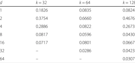
Table 8 lists the best degree distributions obtained by the ECSO-based approach. A common phenomenon about the distributions of degree values can be found: lower degrees possess bigger probabilities. The probability of degree (D= 1) is the biggest and that of degree (D= 2) is the second biggest. Besides, the sum of two probabilities is more than 0.5, which guarantees the success of decod-ing and is in accordance with the characteristic of typical degree distributions such as ISD and RSD.
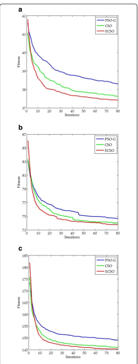
Figure2 shows the merit of the proposed ECSO-based approach in terms of aggressive nature, in which the curves are averaged by the statistical data of 40 runs. It can be observed that both the convergence rate and optimization precision of ECSO are better than those of PSO-G and CSO. In addition, during the optimization
process, the ECSO-based approach can always take the leads with the lowest fitness values when the iteration exceeds 10. For K32, the fitness value of ECSO quickly drops down to 38.0941 when the iteration increases to 20, whereas the fitness values of PSO-G and CSO are 39.4872 and 38.6013, respectively. As the iteration rises to 40, the convergence rates of the three approaches be-come to slow down, but the performance of the ECSO is still the best. For K128, the fitness value of ECSO quickly falls rapidly to 147.1244 when the iteration in-creases to 30, whereas the fitness values of PSO-G and CSO are 152.3841 and 148.8773, respectively. Though the gap between ECSO and CSO is smaller, the gap be-tween ECSO and PSO-G is still considerable. Greater improvement can be expected when thekrises to thou-sands, which is very meaningful to the practical applica-tions of short-length LT codes.
6 Conclusion
Recognizing the design of degree distribution is critical to the DFC-based cooperative communication schemes; this paper proposes an ECSO-based approach for opti-mizing degree distributions of short-length LT codes. Firstly, we establish an optimization framework for the problem on the basis of sparse degree distributions. The search space dimension is reduced to D withdmax= 2D
and the average number of encoded symbols required is chosen to calculate the objective fitness value. Secondly, an enhanced CSO algorithm, termed as ECSO, is de-signed for the problem, in which three strategies, SIB, RCE, and IDE, are suggested to enhance the ability of Table 5Comparison of the optimization solutions with three
algorithms for solving K32
Algorithm Standard deviation
Mean Best Worst
f f f Overhead f Overhead
PSO-G 0.4129 38.3575 37.8000 0.1813 39.8000 0.2438
CSO 0.3382 37.6063 36.6250 0.1445 38.3750 0.1992
ECSO 0.3477 37.4281 36.5000 0.1406 38.0000 0.1875
Table 6Comparison of the optimization solutions with three algorithms for solving K64
Algorithm Standard deviation
Mean Best Worst
f f f Overhead f Overhead
PSO-G 0.8183 74.6711 70.2235 0.0972 77.3750 0.2090
CSO 0.7815 74.0125 69.1326 0.0802 75.6250 0.1816
ECSO 0.7602 73.3750 68.0000 0.0625 75.0000 0.1719
Table 7Comparison of the optimization solutions with three algorithms for solving K128
Algorithm Standard deviation
Mean Best Worst
f f f Overhead f Overhead
PSO-G 1.9759 149.0875 145.0000 0.1328 153.0000 0.1953
CSO 1.3793 146.0437 142.7320 0.1151 148.7500 0.1621
ECSO 1.4517 145.0875 141.0000 0.1016 147.2500 0.1504
Table 8Optimal degree distributions obtained from the ECSO-based approach for solving K32, K64, and K128
d k= 32 k= 64 k= 128
1 0.1826 0.0835 0.0824
2 0.3754 0.6660 0.4676
4 0.2886 0.0822 0.2673
8 0.0817 0.0596 0.0430
16 0.0717 0.0801 0.0667
32 – 0.0286 0.0423
optimization. Thirdly, an ECSO-based approach is de-scribed in detail. Simulation results demonstrate the ef-fectiveness of the three strategies and show that the ECSO-based approach outperforms the PSO-G-based approach and CSO-based approach in terms of optimization efficiency and convergence rate. For the fu-ture work, our research will focus on optimizing degree distribution for unequal error protection (UEP) applica-tion of DFC-based cooperative communicaapplica-tion schemes, by employing novel SI algorithms.
Abbreviations
CSO:Chicken swarm optimization; DFC: Digital fountain code; PLC: Power line communication; PSO: Particle swarm optimization; SDD: Sparse degree distribution; UEP: Unequal error protection
Acknowledgements
There are no other participants in this work except those in the author’s list.
Funding
The research was supported by the technology programme of State Grid Hebei Electric Power Research Institute (No. KJ2017–016).
Availability of data and materials
Data sharing not applicable to this article as no datasets were generated or analyzed during the current study.
Authors’contributions
PL conceived and created the research and then performed simulations and wrote the draft. HF and WS reviewed and corrected the manuscript. QX and ZY performed the simulations and calculations. ZX gave the constructive suggestion. All authors read and approved the final manuscript.
Competing interests
The authors declare that they have no competing interests.
Publisher’s Note
Springer Nature remains neutral with regard to jurisdictional claims in published maps and institutional affiliations.
Author details
1
State Grid Hebei Electric Power Research Institute, Shijiazhuang 050021, China.2School of Electronics and Information Engineering, Tianjin Polytechnic University, Tianjin 300387, China.
Received: 20 August 2018 Accepted: 21 February 2019
References
1. A.W. Kabore, V. Meghdadi, J.P. Cances, in18th IEEE International Symposium on Power Line Communications and Its Applications. Cooperative relaying in narrow-band PLC networks using fountain codes (Glasgow, IEEE, 2014), pp. 306–310
Fig. 2Convergence process of the three approaches for solving
2. S. Ezzine, F. Abdelkefi, J.P. Cances, V. Meghdadi, A. Bouallegue, in2015 IEEE 81st Vehicular Technology Conference (VTC Spring). Capacity analysis of an OFDM-based two-hops relaying PLC systems (Glasgow, IEEE, 2015), pp. 1–5
3. J.W. Byers, M. Luby, M. Mitzenmacher, A. Rege,A digital fountain approach to reliable distribution of bulk data, Proceedings of ACM SIGCOMM (1998), pp. 56–67
4. C.M.C. Pei-Chuan Tsai, Y.P. Chen, in2012 IEEE Congress on Evolutionary Computation. Sparse degrees analysis for LT codes optimization (Brisbane, IEEE, 2012), pp. 1–6
5. M. Luby, inProc. 43rd Symp. Foundations Computer Science (FOCS 2002). LT codes (Vancouver, IEEE, 2002), pp. 16–19
6. A. Shokrollahi, Raptor codes. IEEE Trans. Inf. Theory52(6), 2551–2567 (2006) 7. P. Maymounkov, inNYU Tech. Rep. TR2003–883. Online codes (2002) 8. R. Wang, H. Liang, H. Zhao, G. Fang, Deep space multi-file delivery protocol
based on LT codes. J. Syst. Eng. Electron.27(3), 524–530 (2016) 9. K.h. Lee, C.k. Kim, S.H. Lee, W.t. Kim, in2015 International Conference on Big
Data and Smart Computing (BIGCOMP). Rateless code based reliable multicast for data distribution service (Jeju, IEEE, 2015), pp. 150–156 10. W. Du, Z. Li, J.C. Liando, M. Li, From rateless to distanceless: enabling sparse
sensor network deployment in large areas. IEEE/ACM Trans. Networking 24(4), 2498–2511 (Aug. 2016)
11. C. Anglano, R. Gaeta, and M. Grangetto, Exploiting rateless codes in cloud storage systems, in IEEE Transactions on Parallel and Distributed Systems, 26, 5, pp. 1313–1322, 2015
12. H. Zhu, G. Zhang, G. Li, in2008 11th IEEE International Conference on Communication Technology. A novel degree distribution algorithm of LT codes (Hangzhou, IEEE, 2008), pp. 221–224
13. L. Zhang, J. Liao, J. Wang, T. Li, Q. Qi, Design of improved Luby transform codes with decreasing ripple size and feedback. IET Communication8(8), 1409–1416 (2014)
14. P.C. Tsai, C.M. Chen, Y.P. Chen, in2014 IEEE Congress on Evolutionary Computation (CEC). A novel evaluation function for LT codes degree distribution optimization (Beijing, IEEE, 2014), pp. 3030–3035 15. W. Yao, B. Yi, W. Li, T. Huang, Q. Xie, CPRSD for LT codes. IET
Communication10(12), 1411–1415 (2016)
16. E. Hyytia, T. Tirronen, J. Virtamo, inIEEE INFOCOM 2007 - 26th IEEE International Conference on Computer Communications. Optimal degree distribution for LT codes with small message length (Anchorage, IEEE, 2007), pp. 2576–2580
17. E.A. Bodine, M.K. Cheng, in2008 IEEE International Conference on Communications. Characterization of Luby transform codes with small message size for low-latency decoding (Beijing, IEEE, 2008), pp. 1195–1199 18. E. Hyytia, T. Tirronen, J. Virtamo, inProceedings of the 6th International
Workshop on Rare Event Simulation (RESIM 2006). Optimizing the degree distribution of LT codes with an importance sampling approach (Bamberg, 2006), pp. 64–73
19. S. Jafarizadeh, A. Jamalipour, in2014 IEEE Wireless Communications and Networking Conference (WCNC). An exact solution to degree distribution optimization in LT codes (Istanbul, IEEE, 2014), pp. 764–768
20. J.K. Zao, M. Hornansky, P.-l. Diao, in2012 IEEE Congress on Evolutionary Computation. Design of optimal short-length LT codes using evolution strategies (Brisbane, IEEE, 2012), pp. 1–9
21. C.M. Chen, Y.p. Chen, T.C. Shen, J.K. Zao, inIEEE Congress on Evolutionary Computation. On the optimization of degree distributions in LT code with covariance matrix adaptation evolution strategy (Barcelona, IEEE, 2010), pp. 1–8
22. Z.H. Deng, B.S. Yi, L.C. Gan, J.S. Xiao, C. Huang, Degree distribution design of LT codes using PSO algorithm with gradient. J. Beijing Univ. Posts Telecommun.34(3), 40–43 (2011)
23. X.B. Meng, Y. Liu, X.Z. Gao, H.Z. Zhang, inAdvances in Swarm Intelligence. A new bio-inspired algorithm: Chicken swarm optimization (Springer International Publishing, Berlin, 2014), pp. 86–94
24. G. Sun, Y.H. Liu, S. Liang, Z.Y. Chen, A.M. Wang, Q.A. Ju, Y. Zhang, A sidelobe and energy optimization array node selection algorithm for collaborative beamforming in wireless sensor networks. IEEE Access6, 2515–2530 (2018) 25. D. Wu, S. Xu, F. Kong, Convergence analysis and improvement of the
chicken swarm optimization algorithm. IEEE Access4, 9400–9412 (2016) 26. W. Shi, Y. Guo, S. Yan, Y. Yu, P. Luo, J. Li, Optimizing directional reader
antennas deployment in UHF RFID localization system by using a MPCSO algorithm. IEEE Sensors J.18(12), 5035–5048 (Jun. 2018)
27. R. Storn, K. Price,Differential evolution-a simple and efficient adaptive scheme for global optimization over continuous spaces. Tech. Rep. TR-95-012, (ICSI, USA,1995)
28. R. Storn, K.V. Price, Differential evolution a simple and efficient heuristic for global optimization over continuous space. J. Global Optim11(4), 341–359 (1997) 29. Y. Shi, R. Eberhart, inProc. IEEE Int. Conf. Evol. Comput. A modified particle