R E S E A R C H
Open Access
Scan statistics with local vote for target
detection in distributed system
Junhai Luo
1,2*and Qi Wu
1Abstract
Target detection has occupied a pivotal position in distributed system. Scan statistics, as one of the most efficient detection methods, has been applied to a variety of anomaly detection problems and significantly improves the probability of detection. However, scan statistics cannot achieve the expected performance when the noise intensity is strong, or the signal emitted by the target is weak. The local vote algorithm can also achieve higher target detection rate. After the local vote, the counting rule is always adopted for decision fusion. The counting rule does not use the information about the contiguity of sensors but takes all sensors’ data into consideration, which makes the result undesirable. In this paper, we propose a scan statistics with local vote (SSLV) method. This method combines scan statistics with local vote decision. Before scan statistics, each sensor executes local vote decision according to the data of its neighbors and its own. By combining the advantages of both, our method can obtain higher detection rate in low signal-to-noise ratio environment than the scan statistics. After the local vote decision, the distribution of sensors which have detected the target becomes more intensive. To make full use of local vote decision, we introduce a variable-step-parameter for the SSLV. It significantly shortens the scan period especially when the target is absent. Analysis and simulations are presented to demonstrate the performance of our method.
Keywords: Scan statistics, Target detection, Local vote decision, Data fusion, Variable-step-parameter
1 Introduction
Target detection has an important research significance on military and civil applications in distributed system, such as intrusion detection and fire detection. The relia-bility of target detection result suffers from the problem of local false alarm, while data fusion can improve the precision of the target detection. For multiple sensor sys-tems, sensors send their sense data to a fusion center, and the fusion center makes the final decision to improve the global probability of detection. Distributed detection using multiple sensors and optional fusion rules has been extensively investigated.
Chair and Varshney [1] present an optimum fusion structure to classical Bayesian detection problem in dis-tributed sensor networks. To obtain the global decision, the fusion center weighs the reliability of every sensor and
*Correspondence: [email protected]
1School of Electronic Engineering, University of Electronic Science and Technology of China, No.2006, Xiyuan Ave, West Hi-Tech Zone, 61000 Chengdu, China
2Department of Electrical Engineering and Computer Science, The University of Tennessee Knoxville, 37919 Knoxville, USA
compares them with a threshold. The reliability of sen-sor is supported by the probability of detection and false alarm rate. Although this method can get optimum per-formance, it has to know the probability of detection and false alarm rate previously. Since we cannot get the target location before detection, this method cannot be applied to practical applications.
Niu and Varshney [2] put forward the counting rule, where the fusion center employs the total number of detections reported by local sensors for hypothesis testing and analyzes the performance of the counting rule with a significant number of sensors. In [3], the authors give per-formance analysis when sensors are deployed in a random sensor field. The counting rule does not need the prob-abilities of local detection and a false alarm in advance. It makes the counting rule more suitable for the practical environment. For the counting rule, it takes the results of sensors equally. However, sensors close to the target get higher accuracy than sensors far away. Sensors far away from the target degrade global probability of detection. In [4, 5], the authors propose a method which gives dif-ferent weight to each sensor depending on the evaluated
distance to the target or the signal-to-noise ratio (SNR). It makes the final decision more accurate at the cost of sending more data to the fusion center.
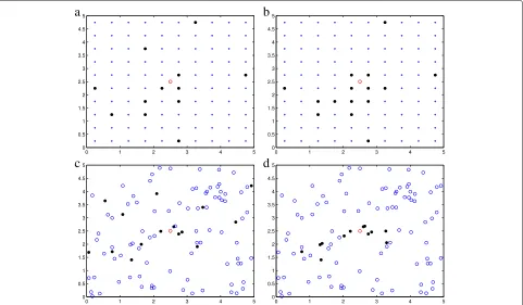
The authors in [6] propose the local vote algorithm using decisions of neighboring sensors and making a col-lective decision as a network. The authors examine both distance-based and nearest neighbor-based versions of local vote algorithm for grid and random sensor deploy-ments and show that in many situations, for a fixed system false alarm, the local vote correction achieves signifi-cantly higher target detection rate than the decision fusion based on uncorrected decisions (see Fig. 1). The authors in [7] propose an improved threshold approximation for the local vote decision fusion and demonstrate that this method can achieve a more accurate result.
Scan statistics has been used to an epidemic or com-puter intrusion in [8–11]. Moreover, Guerriero [12] puts the scan statistics to the signal processing community firstly. The detection is carried out in a mobile fusion center as a mobile agent (MA) which successively counts the number of binary decisions reported by local sensors lying inside its moving field of view. The MA, playing the role of the fusion center, makes the final decision about the presence of a target. The authors also demon-strate the existence of optimal size for the field of view and the disjoint-window test. In disjoint-window scan
test, the MA travels across the sensor network and scans the network using no overlapping windows. In [13–15], the authors introduce the variable window scan statistics and investigate the performance of those variable window scan statistics methods. The disjoint-window scan statis-tics can shorten the scan period. However, it has poor performance compared with the scan statistics (SS).
How to improve the probability of detection while reducing the false alarm rate is an eternal topic. To han-dle complex network environments, improving the global performance in low SNR is our primary goal. The research mentioned above can improve the detection probability and decrease the false alarm rate. However, those algo-rithms cannot meet the expected performance in low SNR. The local vote algorithm can significantly improve the global performance, especially in low SNR. After the local vote, the counting rule is adopted for decision fusion. The counting rule does not consider the spatial correla-tion that sensors near the target have a higher probability of reporting detections. It weakens the advantage which is brought by local vote. In this paper, we combine two previous ideas: local vote decision and scan statistics. Sensors make a local vote, and the MA performs scan statistics. According to Fig. 1, we can see that local vote makes the distribution of sensors which have detected the target more concentrated. It inspires us to introduce a
variable-step-parameter for the scan statistics with a local vote (SSLV). Our contributions in this paper are described as follows.
• A model of the SSLV is proposed. We analyze the
difference between the SSLV and the traditional SS. The deduction of global false alarm ratio for the SSLV is developed.
• We apply the SSLV to a grid sensor network and
compare its performance with the SS. According to the simulation, we can prove that the SSLV
overwhelms the SS in low SNR. We also verify that an optimalMxat a given situation does exist.
• We introduce a variable-step-parameter for the SSLV
and analyze its influence on our method. From the simulation, we know that the variable-step-parameter has little negative effect on detection performance of the SSLV. However, it significantly shortens the scan period especially when a target is absent.
The remainder of the paper is organized as follows. Section 2 demonstrates two-dimensional scan statistics as a foundation for the SSLV. Section 3 describes the system model of scan statistics with the local vote and intro-duces a variable-step-parameter into the SSLV. Section 4 applies the SSLV to a grid sensor network, and various simulations and analysis are provided. Finally, Section 5 concludes our research.
2 Scan statistics
In this part, we will introduce the classical two-dimensional scan statistics algorithm. The scan statistics is a kind of distributed detection method. Each sensor makes its hypotheses according to its sense data and sends the result to the fusion center. The traditional counting rule algorithm collects data from all sensors in the field of interest and makes the global judgment through these data. Unlike the counting rule algorithm, the SS makes an MA sequentially collect the data from the agent area, and the MA makes the final decision for the global network. When a target is present, sensors near the target are more likely to make the right judgments. The SS considers this spatial correlation that makes it more accurate than the counting rule.
We assume that all sensors follow the same hypothe-ses: eitherH0(target absent) is valid orH1(target present) is uniformly accurate. R presents the region of interest (ROI). We deploy sensors in region R , and the region is defined by [0,T1] × [0,T2]. More specifically, let hi = Ti/Ni > 0, whereNiare positive integers, and
i = 1, 2. For 1 ≤ i ≤ N1and 1 ≤ j ≤ N2, letXi,jbe
the count of sensors that have been observed in the rect-angular basic regions [(i − 1)h1,ih1] ×
(j − 1)h2,jh2
. In the process of scan, the MA records the results of
sum in its agent region, and the size of agent region is
m1bym2. respectively. We also call them1andm2the window sizes of the MA. The MA collects data and finds the maximum value to compare with a pre-set threshold valuek.
Sm1×m2N1×N2 =max{vi1,i2; 1 ≤ i1 ≤ N1 − m1 +1, 1 ≤ i2 ≤ N2 − m2 + 1} (2) If there is a maximum value greater thank, we can say that k events are clustered within the inspected region. Therefore, the global probability of detection PD and global probability of false alarm PF can be respectively expressed as
It is important for us to give the expression of
PSm1×m2N×N ≥ k
. Although there is no exact expression for PSm1×m2N1×N2 ≥ k
, we can eval-uate the approximation for it. When the Xij is the Bernoulli random variable with parameter P = α, where 0 < α < 1, the accurate approximation for
PSm1×m2N1×N2 ≥ k
The full content can be found in [12, 16]. In [12], the authors also demonstrate the expression when the Xi,j
conforms to Poisson distribution.
3 Two-dimensional scan statistics with local vote decision
3.1 Scan statistics with local vote decision
Precisely, in this part, we will give an introduction about the SSLV in two-dimensional region. The underlying assumptions in the last part are still suitable here. The dif-ference is that we let sensors make a local vote decision before scan statistics. According to [6], we can take vari-ous neighborhood algorithms, such as fixed distanceror fixed size. Any one of those algorithms can be selected, then all corresponding parameters can be confirmed. For better description, we will redefine some variables. LetXi,j
be the event that has been observed in the rectangular sub-regions [ih1,(i + 1)h1]×
and for simplicity, we exclude the rectangular sub-regions on the edge of the field in this part. For 1 ≤ i ≤ N1 makes the final decision that a target is present. The largest number of events in an agent region can be expressed as
Sm1×m2;N1z×N2 = max {vi1,i2; 1 ≤ i1 ≤ N1 − m1 +1, 1 ≤ N2 − m2 + 1} (6) For simplicity, we abbreviate Sm1×m2;N1×N2 to S. The next step is to obtain the expression of
PSm1×m2N×N ≥ k
to make the SSLV useful.
3.2 Correlation of sensors
Our algorithm introduces local vote decision into the tra-ditional scan statistics. Therefore, we should figure out what has changed after the combination of two algo-rithms. The dependence among sensors should be exam-ined first. For any sensor detection eventZi, we start by
calculating the expected valueμiand varianceσi2of the
updated decision.
where Mi is the number of neighbors which depends
on local vote decision algorithm. Mx is a variable
that has a significant influence on the performance. σi2 = μi(1 − μi).
The dependence betweenZi andZjhas relations with
the intersection of their respective neighborhoods U(i)
andU(j). The number of sensors in the intersectionU(i)∩ U(j)can be denoted byni,j. According to the expression of
covariance, we first computeE(ZiZj) = P(Zi = Zj = 1)
and then calculate the covariance betweenZiandZj. We
divide the neighborhoods into three parts. Suppose that A is the number of positive decisions inU(i)∩U(j)and B is The covariance is then given by
Cov(Zi,Zj) =
E(Zi,Zj) − μiμj
I(ni,j>0) (11)
According to the deductions above, we can find out that decisionXi,jis not i.i.d anymore after the local vote.
3.3 Approximation forP(S ≥ k)
In [16], the authors give the proof of approximation when theXi,jis i.i.d with the Markov Chain imbeddable systems
[17]. Obviously, it is not applicable here. Luckily, there are different ways to give the accurate approximation for
P(S ≥ k)and one of them is using the Haiman theorem [18–20].
Theorem 1Let {Xi} be a stationary 1-dependent
sequence of r.v’s and for x < w, w = sup{u;P(X1≤u) <
N1 = K m1andN2 = Lm2, whereKandLare positive Then, if 1-Q2 ≤ 0.025, we can get approximation from Haiman theorem
P(S ≤ n)≈(2Q2 − Q3)[ 1 + Q2 − Q3 + 2(Q2−Q3)2]−(K−1)
(14)
with an error of about 3.3(K − 1)(1 − Q2)2. To evalu-ate (15), one needs approximations forQ2andQ3. Hence, the question is transformed into evaluating Q2 andQ3. We may apply Theorem 1 again considering the two sequences of random variables defined by
Yl= max
which are also stationary and 1-dependent. Put Q22 = P(Y1≤n),Q23 = P(Y1 ≤n,Y2≤n),Q32 =P(Z1 ≤ n) get the approximations from Theorem 1.
Q2≈(2Q22−Q23)
Assuming thatL ≤ Kand substituting (17) and (16) into (15), we can get the final expression we need.
The total error on the resulting approximation of
P(S ≤ n)is bounded by about
Eapp =3.3(L−1)(K − 1)((1 − Q22)2 + (1 − Q32)2
+(L−1)(Q22−Q23)2). (17)
The exact formulas for Quv,u,v ∈ {2, 3} is hard to
be obtained. Thus, we can use Monte Carlo simulation to evaluate these quantities. The final expression can be given by
P(S≥k)=1−P(S<k)=1−P(S≤k−1) (18)
whereP(S≤k − 1)can be approximated by (15).
3.4 The SSLV with variable-step-parameter
The traditional scan statistics is a kind of continuous scan. Disjoint-window scan statistics means the MA trav-els across the ROI and scans the area using no over-lapping windows. In [12], the authors investigate the disjoint-window test and compare its performance with the scan statistics. Obviously, the scan statistics over-whelms the disjoint-window, and its performance is more stable. However, the disjoint-window can shorten scan period. In this section, we will introduce a variable-step-parameter for the SSLV. In the process of scan, the MA makes a choice for the next start position according to the result of the current scan. Since the detection probability is based on the distance between the target and sensors, sensors near the target have a higher probability of detect-ing the target. If the result of detection is small, we can magnify the value of step to avoid the redundant scan especially when the target is absent. The variable step is given by
The scan region can be a rectangular region given by
R(i1,i2) = [i1h1,(i1 + m)h1] × [i2h2,(i2 + m)h2]. Assuming R(i1,i2) is the scan region at the current time, then the next scan region is
R[(i1+step)h1,(i1+step+m)h1]×[i2h2,(i2 + m)h2], i1+step ≤N − m + 1. We only introduce the step at one-dimensional field for better performance. Whereas, the global false alarm rate can still be evaluated by (15).
4 Application of the SSLV in distributed system In this section, we apply the SSLV into a particular sit-uation and provide a detailed description concerning observation model, local vote decision model, false alarm probability at the MA, and the optimalMx.
4.1 Observations model
in Fig. 1a and in a random pattern in Fig. 1c. We con-sider the two-dimensional field is a square of areasb2. The number of total sensors can be expressed asM.(xs,ys)for
s=1,. . .Mpresent the coordinates of sensors. The coor-dinate of each sensor is known. Noises at local sensors are i.i.d and follow the Gaussian distribution with zero mean and varianceσw2.
ws∼N(0,σw2)s = 1,. . .M (20)
We design each sensorsto decide between the following hypotheses
H0:rs = ws
H1:rs = ys+ws (21)
wherersis the received signal at sensor s. Sensors make
their decisions according to the value ofrs.ys = as/ds ,
andasis i.i.d which follows the Gaussian distribution with
zero mean and varianceσ2(σ2represents the power of the signal that is emitted by the target at distanceds = 1m),
anddsis the Euclidean distance between the local sensor
sand the target
ds =
(xs − xt)2 + (ys − yt)2 (22)
and (xt,yt) are the unknown coordinates of the target.
Sensors near the target receive more signals than those far away. Receiving more signals means higher probabil-ity of detection. In our simulations, we assume that the location of the target follows a uniform distribution, and all local sensors make their judgments by using the same threshold τ. According to the Neyman-Pearson lemma [21], the local sensor-level false alarm rate and probability of detection can be respectively obtained by
pfa = 2Q τ
4.2 Local vote decision model
We divide the ROI intoM(the total number of sensors) little sub-squares. The location of the sensor inside each small sub-square is known. Leth = b/N, whereN sat-isfiesN2 = M, and we divide the square of areab2into M cells so that each cell of areah2contains only one sen-sor. Let us denote the cell [ih,(i + 1)h] × jh,(j + 1)h
byc(i,j). We defineXi,jas the binary data from the local
sensor s inside c(i,j) with 0 ≤ i ≤ N-1 and 0 ≤
j ≤ N-1.
If sensors are deployed along a regular grid, sensors at the vertex of a square can be selected as the neighbors for
local vote algorithm. The number of the neighbors is fixed. Each sensor contains nine neighbors (including itself ) in our simulation. When sensors are randomly deployed in the field, sensors within a fixed distance can be selected as neighbors for local vote algorithm. The number of the neighbors is not fixed in this version. Every sensor receives the decision from its neighbors ignoring the sensors on the edge of the field. If the sum of these decisions exceeds the given thresholdMx, the sensor makes the decision of
target presence. After the local vote decision, the local sensor-level false alarm rate and probability of detection are given by
whereMiis the number of neighbors andMxis the pre-set
threshold. We defineXi,jas the binary data from the local
sensorsinsidec(i,j)with 1≤i≤Nand 1≤j≤Nafter local vote whereN = N−2. We observe that for each 1 ≤ i ≤ N, the sequence(Xi,j)1≤i≤N isc-dependent,
and for each 1 ≤ j ≤ N , the sequence(Xi,j)1≤j≤N
is also c-dependent, where c = 2 in our simulation. c
has relations with the choice of local vote algorithm. In (15), we construct a 1-dependent sequence to evaluate global false alarm probability. Only whenc ≤ mcan we guarantee the sequence is 1-dependent.
4.3 False alarm probability at the MA
The binary data from local sensors can be expressed as
Is = {0, 1}
s = 1,. . .,M.Mrepresents the number of all sensors except those on the edge of the field. When there is a detected target,Istakes the value 1; otherwise, it
takes the value 0 after the local vote. It is easy to verify that
M
The MA travels across the area and sequentially collects the local binary decisions from sensors located inside its agent region, which we consider to be squares of sizefovh.
fovis the size of the window. The sequential fusion rule at
the MA for 1 ≤ i1 ≤ N−fov+1 and 1 ≤ i2≤N−fov+1
is given by
vi1,i2 ≥ k ⇒decide H1
otherwise ⇒MA continues to scan (28)
wherevi1,i2 =
i2+fov+1
j=i2
i1+fov+1
i=i1 Xij. At the MA, the probability of global false alarmPFis
We note that (30) can be evaluated using the approx-imation as in (15) after substituting fov with m andpfa
withα.
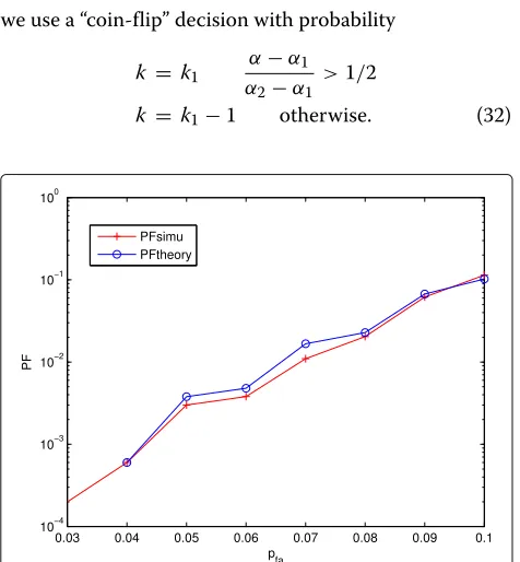
In Fig. 2, we plot the global probability of false alarm
PFfor the MA versus the local probability of false alarm
pfafor the sensor. The curves obtained by using the SSLV
approximation in (15) and simulations (based on 5000 Monte Carlo runs) are plotted. Fig. 2 shows that the approximation in (15) is very accurate.
4.4 OptimalMx
Obviously, the global probabilities of false alarm and detection have relations with the value of Mx. In this
section, we are looking for the optimalMxand trying to
show the existence of optimal value. The choice of Mx
must maximize the probability of detection at the given global false alarm rate so the expression can be written as
max
Mx:PF=αPD (30) wherePDis the probability of detection at the MA. For the given exact value ofα, it is hard to confirm the related parameterkaccording toαbecause it involves dis-crete distributions. To solve this constrained optimization problem in (31), we should use a randomized test [22]. By definingα1andα2as follows
PSfov×fov≥k1
≈α1< α PSfov×fov≥k1−1
≈α2> α, (31)
we use a “coin-flip” decision with probability
k = k1 α−α1 α2−α1 >1/2
k = k1−1 otherwise. (32)
Fig. 2Probability of false alarm for MA PF versus probability of false alarm for the local sensorpfa. Here, we haveN= 27,b= 5,σ2= 1,σw2 = 4,k= 6,Mx= 4, andfov= 5. Simulations are based on 5000 runs
We can confirm the parameterkaccording to the short-est distance fromαtoα1andα2.
When an Mx and the exact global probability of false
alarm is given, we can get the correspondingk. The global probability of detection can be confirmed byk. In Fig. 3, combining with (3) and (30), we plot the global probabil-ity of detection versusMx. α is set to be 0.1. As shown
in Fig. 3, there does exist an optimalMx that maximizes
the probability of detectionPDfor the MA at the given condition. By employing this optimumMx, a significant
improvement inPDcan be achieved. In our simulation, with the increase of Mx, PD increases as well. When
Mx = 4, PD reaches the maximum. After that, PD
decreases with the increase of Mx. The optimalMx has
relations with other parameters and is different in differ-ent environmdiffer-ents. However, under the given condition, there is indeed an optimal value that maximizesPD.
From the perspective of the theory, the increase ofMx
decreases the value ofkfor fixedα. The decrease ofkcan increasePD, meanwhile, the increase ofMxcan decrease
pdsfrom (27). The decrease ofpdsconstrains the increase of PD, and PD mainly relies on pds. The decrease of k
can compensate the influence which is brought by the decrease of pds at the beginning. Hence, PD shows the unimodal characteristic.
5 Performance analysis
After all above analysis, we should compare the SSLV with the scan statistics and find out the difference in perfor-mance between them. Numerous simulations and analysis are given in this section.
In Fig. 4, we plot the global probability of false alarm for the MA versus the thresholdkunder different deploy-ments. In Fig. 4a, sensors are deployed along the regular
Fig. 3Probability of detection for MA versusMx. Here, we have N= 27,b= 5,σ2= 1,σ
Fig. 4Probability of false alarm for MA versus thresholdk. Here, we haveN= 27,b= 5,σ2=1,σ
w2= 4,pfa= 0.05, andfov= 5. Simulations are based on 5000 runs.aGrid deployment.bRandom deployment
grid, and Mi = 9. In Fig. 4b, sensors are randomly
deployed in the field, and the neighborhood distance is set to be 0.1. We can see from Fig. 4 that with the increase of
Mx, the global probability of false alarm decreases
signifi-cantly. What we need is to get lower false alarm rate. There is a crossing point in Fig. 4, which means the scan statis-tics has the same global probability of false alarm with the SSLV at that point. Before that critical point, the SSLV gets a lower PF than the scan statistics. After that, the scan statistics overwhelms the SSLV. It is because the local vote increases the count of sensors that has detected event compared with the scan statistics. This critical point is not an integer and does not exist in fact. However, the near-est two positive integers of crossing point are the practical key points.
In Fig. 5, we plot the global probability of detection for the MA versus the threshold k. From Fig. 5, we know thatPDof the SSLV does not always overwhelm the scan statistics. However, it shows that for the large value of the thresholdk, the SSLV performs better than the scan
Fig. 5Probability of detection for MA versus the thresholdk. Here, we haveN= 27,b= 5,σ2= 1,σ
w2= 4,pf= 0.05, andfov= 5. Simulations are based on 5000 runs.aGrid deployment.bRandom deployment
statistics. The larger thresholdkmeans the smaller global probability of false alarm is demanded. It is related to the value ofMx. With the increase ofMx, we get lower false
alarm rate; however, the probability of detection decreases as well. Hence, it is important to select the value ofMx
according to the various detection environments. At the given condition, we can use the method in Section 3.4 to evaluate the optimalMx. Overall, the SSLV can
substan-tially decrease the probability of false alarm and improve the global probability of detection compared with the scan statistics.
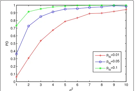
In Fig. 6, we plot the global probability of detection for the MA versus σ2 (power of the signal that is emitted by the target at a distanceds = 1 m) at different local
Fig. 6Probability of detection for MA versusσ2. Here, we haveN= 27, b= 5,Mx= 3,σw2= 6, andfov= 5. Simulations are based on 5000 runs
In Fig. 7, we plot the global probability of detection ver-susσ2for different methods. Figure 7 illustrates the SSLV has higherPDthan scan statistics when the SNR is low. It means our SSLV is more suitable for the tough environ-ment. When the SNR is high, the advantage of the SSLV is not evident.
After introducing a variable-step-parameter into the SSLV, we should figure out its influence on the SSLV. Figure 8 presents the receiver operating characteristic curves (ROC) of the SSLV and the SSLV with the variable-step-parameter. From Figure 8, we can see that the variable-step-parameter has little negative effect on the performance of detection. The local vote makes the dis-tribution of sensors report event so concentrated that we can use this parameter without worry. Figure 9 shows the scan times of different methods to show the advantage
Fig. 7Probability of detection for MA versusσ2. Here, we have N= 27,b= 5,σw2= 4,k= 8,pfa= 0.05, andfov= 5. Simulations are based on 5000 runs
Fig. 8ROC of SSLV and SSLV with variable step. Here, we have N= 27,b= 5,σ2= 1,σ
w2= 4,pfa= 0.05,k= 6,Mx= 3, andfov= 5. Simulations are based on 5000 runs
of variable-step-parameter. When the target is absent, the SSLV with variable step significantly decreases the times of scan, meanwhile, when the target is present, the SSLV with variable step reduces the times of scan to some extent. In our simulation, the target is placed at the center of the field.
6 Conclusions
This paper has introduced the SSLV algorithm specially designed to work with target detection in low SNR condi-tion. The correlation between sensors and the expression for global false alarm ratio after the local vote have been described in detail. Moreover, based on the SSLV, the SSLV with variable-step-parameter has been proposed. The two algorithms have been examined in simulation
studies which revealed that they produce similar detec-tion accuracies, but the SSLV with variable step method is substantially faster during once scan cycle. Nevertheless, there are some potential research topics which will be fur-ther discussed. Firstly, it is evident that getting the optimal
Mx from the simulation is not the optimal method and
a new expression for the optimalMx should be deduced.
Furthermore, the variable-step-parameter for the SSLV can be extended to two-dimensional without losing any detection performance.
Acknowledgements
This work was supported in part by the Overseas Academic Training Funds, University of Electronic Science and Technology of China (OATF, UESTC) (Grant No.201506075013), and the Program for Science and Technology Support in Sichuan Province (Grant Nos. 2014GZ0100 and 2016GZ0088).
Authors’ contributions
JHL and QW proposed the algorithm and carried out the simulations. JHL and QW analyzed the experimental results. JHL gave the critical revision and final approval. Both authors read and approved the final manuscript.
Competing interests
The authors declare that they have no competing interests.
Publisher’s Note
Springer Nature remains neutral with regard to jurisdictional claims in published maps and institutional affiliations.
Received: 7 December 2016 Accepted: 21 April 2017
References
1. Z Chair, PK Varshney, Optimal data fusion in multiple sensor detection systems. IEEE Trans. Aerosp Electron Syst.22(1), 98–101 (1986) 2. R Niu, PK Varshney, MH Moore, D Klamer,Decision fusion in a wireless
sensor network with a large number of sensors. presented at the 7th IEEE Int. Conf. Information Fusion (ICIF). (Stockolm, Sweden, 2004)
3. R Niu, P Varshney, Performance analysis of distributed detection in a random sensor field. IEEE Trans. Signal Process.56(1), 339–349 (2008) 4. D Marco, Y-H Hu, Distance-based decision fusion in a distributed wireless
sensor network. Telecommun Syst.26(2–4), 339–350 (2004) 5. SH Javadi, A Peiravi, Fusion of weighted decisions in wireless sensor
networks. IET Wirel Sens. Syst.5(2), 97–105 (2015)
6. N Katenka, E Levina, G Michailidis, Local vote decision fusion for target detection in wireless sensor networks. IEEE Trans. Signal Process.56(1), 329–338 (2008)
7. MS Ridout, An improved threshold approximation for local vote decision fusion. IEEE Trans. Signal Process.61(5), 1104–1106 (2013)
8. T Tango, K Takahashi, A flexible spatial scan statistic with a restricted likelihood ratio for detecting disease clusters. Stat. Med.31(30), 4207 (2012)
9. J Fu, W Lou,Distribution theory of runs and patterns and its applications. (World Scientific, Singapore, 2003)
10. DU Pfeiffer, KB Stevens, Spatial and temporal epidemiological analysis in the Big Data era. Prev. Vet. Med.122(1–2), 213–220 (2015)
11. C Teljeur, A Kelly, M Loane,et al,Using scan statistics for congenital anomalies surveillance: the EUROCAT methodology, vol. 30, (2015), p. 1165 12. M Guerriero, P Willett, J Glaz, Distributed target detection in sensor
networks using scan statistics. IEEE Trans. Signal Process.57(7), 2629–2639 (2009)
13. TL Wu, J Glaz, A new adaptive procedure for multiple window scan statistics. Comput. Stat. Data Anal.82(82), 164–172 (2015) 14. BJ Reich, Multiple window discrete scan statistic for higher-order
Markovian sequences. J. Appl. Stat.42(8), 1–16 (2015)
15. X Wang, J Glaz, Variable window scan statistics for normal data. Commun. Statistics-Theory Methods.43, 2489–2504 (2014)
16. MV Boutsikas, M Koutras, Reliability approximations for Markov chain imbeddable systems. Method. Comput. Appl. Probab.2, 393–412 (2000) 17. WC Lee, Power of discrete scan statistics: a finite Markov chain imbedding
approach. Methodol. Comput. Appl. Probab.17(3), 833–841 (2015) 18. A Amarioarei, C Preda, Approximations for two-dimensional discrete scan
statistics in some block-factor type dependent models. J. Stat. Plann. Infer.
151(3), 107–120 (2014)
19. G Haiman, C Preda, Estimation for the distribution of two-dimensional discrete scan statistics. Methodol. Compu. Appl. Probab.8(373), 382 (2006) 20. G Haiman, 1-dependent stationary sequences for some given joint
distributions of two consecutive random variables. Methodol. Comput. Appl. Probab.14, 445–458 (2012)
21. HV Poor, An introduction to signal detection and estimation. Springer Texts Electr. Eng.333(1), 127–139(13) (1998)
22. S Kotz, DL Banks, CB Read,Read, Encyclopedia of statistical sciences. (Wiley-Interscience, New York, 1997)
Submit your manuscript to a
journal and benefi t from:
7Convenient online submission 7Rigorous peer review
7Immediate publication on acceptance 7Open access: articles freely available online 7High visibility within the fi eld
7Retaining the copyright to your article