Synthesized grain size distribution in the interstellar medium
Hiroyuki Hirashita1and Takaya Nozawa2
1Institute of Astronomy and Astrophysics, Academia Sinica, P.O. Box 23-141, Taipei 10617, Taiwan
2Kavli Institute for the Physics and Mathematics of the Universe, Todai Institutes for Advanced Study, the University of Tokyo, Kashiwa, Chiba 277-8583, Japan
(Received November 7, 2011; Revised March 15, 2012; Accepted March 16, 2012; Online published March 12, 2013)
We examine a synthetic way of constructing the grain size distribution in the interstellar medium (ISM). First, we formulate a synthetic grain size distribution composed of three grain size distributions processed with the following mechanisms that govern the grain size distribution in the Milky Way: (i) grain growth by accretion and coagulation in dense clouds, (ii) supernova shock destruction by sputtering in diffuse ISM, and (iii) shattering driven by turbulence in diffuse ISM. Then, we examine if the observational grain size distribution in the Milky Way (called MRN) is successfully synthesized or not. We find that the three components actually synthesize the MRN grain size distribution in the sense that the deficiency of small grains by (i) and (ii) is compensated by the production of small grains by (iii). The fraction of each contribution to the total grain processing of (i), (ii), and (iii) (i.e., the relative importance of the three contributions to all grain processing mechanisms) is 30–50%, 20–40%, and 10–40%, respectively. We also show that the Milky Way extinction curve is reproduced with the synthetic grain size distributions.
Key words:Cosmic dust, interstellar medium, grain size distribution, extinction, Milky Way.
1.
Introduction
Dust grains are important in some physical processes in the interstellar medium (ISM). For example, they domi-nate the absorption and scattering of the stellar light, af-fecting the radiative transfer in the ISM. The extinction (absorption+scattering) by dust in the ISM as a function of wavelength is called the extinction curve (Wickramasinghe, 1967; Hoyle and Wickramasinghe, 1991; Draine, 2003 for review). Extinction curves are important not only in ba-sic radiative processes in the ISM, but also in interpret-ing observational data: part of stellar light in a galaxy is scattered, or absorbed, by dust grains within the galaxy in a wavelength-dependent way according to the extinc-tion curve. Therefore, to derive the intrinsic stellar spec-tral energy distribution of a galaxy, we always have to cor-rect for dust extinction by considering the extinction curve (Calzetti, 2001).
Extinction curves generally reflect the grain composition and the grain size distribution. Mathis et al.(1977, here-after MRN) show that a mixture of silicate and graphite dust, as originally proposed by Hoyle and Wickramasinghe (1969), with a grain size distribution (number of grains per grain radius) proportional toa−3.5, whereais the grain ra-dius (a ∼0.001–0.25μm), reproduces the Milky Way ex-tinction curve. Pei (1992) shows that the exex-tinction curves in the Magellanic Clouds are also explained by the same power-law grain size distribution (i.e.,∝a−3.5) with
differ-ent abundance ratios between the silicate and graphite. Kim
Copyright cThe Society of Geomagnetism and Earth, Planetary and Space Sci-ences (SGEPSS); The Seismological Society of Japan; The Volcanological Society of Japan; The Geodetic Society of Japan; The Japanese Society for Planetary Sci-ences; TERRAPUB.
doi:10.5047/eps.2012.03.003
et al.(1994) and Weingartner and Draine (2001) have ap-plied a more detailed fit to the Milky Way extinction curve in order to obtain the grain size distribution. Although their grain size distributions deviate from the MRN size distri-bution, the overall trend from small to large grain sizes roughly follows a power law with an index near to−3.5. Therefore, the MRN grain size distribution is still valid as a first approximation of the interstellar grain size distribution in the Milky Way.
What regulates or determines the grain size distribution? There are some possible processes that actively and rapidly modify the grain size distribution. Hellyer (1970) shows that the collisional fragmentation of dust grains finally leads to a power law grain size distribution similar to the MRN size distribution (see also Bishop and Searle, 1983). In fact, Hirashita and Yan (2009) show that such a fragmentation and disruption process (or shattering) can be driven effi-ciently by turbulence in the diffuse ISM. However, they also show that grain velocities are strongly dependent on grain size; as a result, the grain size distribution does not converge to a simple power-law after shattering. Moreover, dust grains are also processed by other mechanisms. Vari-ous authors show that the increase of dust mass in the Milky Way ISM is mainly governed by grain growth through the accretion of gas phase metals onto the grains (elements comprised of dust grains are referred to as “metals”) (Dwek, 1998; Inoue, 2003; Zhukovskaet al., 2008; Draine, 2009; Inoue, 2011; Asano et al., 2013). In the dense ISM, co-agulation also occurs, making the grain sizes larger (e.g., Hirashita and Yan, 2009). In the diffuse ISM phase, in-terstellar shocks associated with supernova (SN) remnants (simply called SN shocks in this paper) destroy dust grains, especially small ones, by sputtering (e.g., McKee, 1989).
Shattering also occurs in SN shocks (Joneset al., 1996). Modeling the evolution of the grain size distribution in the ISM is a challenging problem because a variety of processes are concerned as mentioned above. Those pro-cesses are also related to the multi-phase nature of the ISM. Liffman and Clayton (1989) calculate the evolution of grain size distributions by taking into account grain growth and shock destruction. However, their method could not treat disruptive and coagulative processes (i.e., shattering and co-agulation). O’Donnell and Mathis (1997) also model the evolution of grain size distribution in a multi-phase ISM, taking into account shattering and coagulation, in addition to the processes considered in Liffman and Clayton (1989). They use the extinction curve and the depletion of gas-phase metals as quantities to be compared with observations. Al-though their models are broadly successful, the fit to the ul-traviolet extinction curve is poor, which they attribute to the errors caused by their adopted optical constants. They also show that inclusion of molecular clouds in addition to dif-fuse ISM phases improves the fit to the observed depletion, but they did not explicitly show the effects of molecular clouds on the extinction curve. Yamasawaet al. (2011) have recently calculated the evolution of the grain size distribu-tion in the early stage of galaxy evoludistribu-tion by considering the ejection of dust from SNe and subsequent destruction in SN shocks. Since they focus on the early stage, they did not include other processes such as grain growth and disrup-tion (shattering), which are important in solar-metallicity environments such as in the Milky Way (Hirashita and Yan, 2009).
Comparing theoretical grain size distributions with ob-servations is not a trivial procedure. In a line of sight, we always observe a mixture of grains processed in various ISM phases. Therefore, a “synthetic” grain size distribu-tion, which is made by summing typical grain size distri-butions in individual ISM phases with certain weights, is to be compared with observations. In this paper, we first formulate a synthetic way of reproducing the grain size dis-tribution. Then, we carry out a fitting of synthetic grain size distributions to the observational grain size distribution, in order to obtain the relative importance of individual grain processing mechanisms. We do not model the multi-phase ISM in detail, but our fitting contains the information on the weights (i.e., relative importance) of different grain pro-cessing mechanisms, which depend on the ISM phase.
This paper is organized as follows. In Section 2, we explain our synthetic method to reconstruct the grain size distribution in the ISM. In Section 3, we fit our synthetic models to the observational grain size distribution in the Milky Way, and examine if the fitting is successful or not. In Section 4, after we discuss our results, we calculate the extinction curves to examine if our synthesized grain size distributions are consistent with the observed extinction or not. In Section 5, we give our conclusions.
2.
Synthetic Grain Size Distribution
As explained in Introduction, we “synthesize” the obser-vational grain size distribution (here, the MRN size bution) by summing some representative grain size distri-butions in various ISM phases. These representative grain
size distributions are explained in Subsection 2.1.
First, the ISM is divided into two parts: one is the part where the grain processing is occurring (called the “grain-processing region”), and the other is the area where the grains already processed in the various grain-processing re-gions are well mixed (called the “mixing region”). The mass fractions of the former and the latter regions are, re-spectively, fprocand 1−fproc. It is reasonable to assume that
the grain size distribution in the mixing region should be the mean grain size distribution in the ISM (Subsection 2.2).
We assume that all grains are spherical with material density s; thus, the grain mass m is expressed as m =
4 3πa
3s. Although coagulation may produce porous grains
(e.g., Ormelet al., 2009), we neglect the effects of porosity and assume all grains to be compact. Two grain species are treated in this paper; silicate and graphite. To avoid com-plexity arising from compound species, we treat these two species separately. This separate treatment is also practi-cal in this paper as we (and other authors usually) assume that the observed extinction curve can be fitted with the two species (Subsection 4.4). Before being processed, the grain size distribution is assumed to be MRN: a power-law func-tion with power index−r (r =3.5), and upper and lower bounds for the grain radii (whose values are determined be-low)aminandamax, respectively:
nMRN(a)=
0. The grain size distribution is defined so thatnMRN(a)da
is the number of grains whose sizes are between a and
a+daper hydrogen nucleus. The dust mass density, ρd,
is related to the metallicityZ(the mass fraction of elements heavier than helium in the ISM) and the hydrogen number densitynHas (Hirashita and Kuo, 2011)
ρd=
for silicate and C for graphite), fXis the mass fraction of X
in the dust,ξ is the fraction of element X in the gas phase (i.e., the fraction 1−ξ is in the dust phase), and (X/H) is the solar abundance relative to hydrogen in the number density. The metallicity is assumed to be solar (Z =Z).
We fix the maximum grain radius asamax = 0.25 μm
(MRN). Although the lower bound of the grain size is poorly determined from the extinction curve (Weingartner and Draine, 2001), we assume thatamin =0.3 nm, since a
(C/H) = 3.63×10⁻⁴. We assume that Si occupies a
mass fraction of 0.166 (fX = 0.166) in silicate, while C
is the only element composing graphite (fX = 1). We
adopt s = 3.3 and 2.26 g cm−3 for silicate and graphite,
respectively.
By using the MRN size distribution as the initial con-dition, we calculate the evolution of grain size distribu-tion by the various processes treated in Subsecdistribu-tion 2.1. In the numerical calculation, the grains outside the radius range between amin and amax are removed from the
cal-culation (the removed mass fraction is < 1%). The pro-cesses considered are (i) “grain growth”—grain growth by accretion and coagulation in a dense medium, (ii) “shock destruction”—destruction by sputtering in SN shocks, and (iii) “grain disruption”—grain disruption by shattering in interstellar turbulence. Shattering in SN shocks (Joneset al., 1996) could be included as a separate component, but in our framework, it is not possible to separately constrain the contributions from the two shattering mechanisms because both shattering mechanisms (turbulence and SN shocks) se-lectively destroy grains with a 0.03 μm and increase smaller grains, predicting similar grain size distributions. Thus, we simply assume that the size distribution of shat-tered grains, whatever the shattering mechanism may be, is represented by the one adopted in Subsection 2.1.3.
Although our fitting procedures are based on grain size distributions, we should keep in mind that observational constraints on the grain size distribution are mainly ob-tained by extinction curves. Weingartner and Draine (2001) performed a detailed fit to the Milky Way extinction curve. However, the grain size distributions derived by them broadly follow an MRN-like power law, although there are bumps and dips at some sizes. We will examine the consis-tency with the extinction curve later in Subsection 4.4. 2.1 Processes considered
2.1.1 Grain growth Grain growth occurs in the dense ISM, especially in molecular clouds, through the accretion of metals (called accretion) and the sticking of grains (called coagulation). The change of grain size distri-bution by grain growth has been considered in our previous paper (Hirashita, 2012). The grain size distribution after grain growth is denoted asngrow(a,tgrow), wheretgrowis the
duration of grain growth. We adopttgrow =10 and 30 Myr
based on a typical lifetime of molecular clouds (e.g., Ladaet al., 2010). The metallicity in the Milky Way is high enough to allow the complete depletion of grain-composing mate-rials into dust grains in∼10 Myr. Thus, the total masses of silicate and graphite become 1.33 (= 1/0.75) and 1.18 (=1/0.85) times as large as the initial values, respectively (recall that the dust mass becomes 1/(1−ξ)times as much if all the dust grains accrete all the gas-phase metals). The difference in the grain size distribution betweentgrow=10
and 30 Myr is predominantly caused by coagulation rather than accretion.
2.1.2 Shock destruction We calculate the change of grain size distribution by SN shock destruction in a medium swept by an SN shock, following Nozawa et al. (2006). All SN explosions are represented by an explosion of a star which has a mass of 20 Mat the zero-age main sequence, and the SN explosion energy is assumed to be 1051erg. For
the ISM, we adopt a hydrogen number density of 0.3 cm−3
(since the destruction is predominant in the diffuse ISM; McKee, 1989), and solar metallicity. The calculation of grain destruction is performed until the shock velocity is decelerated down to 100 km s−1 (8×10⁴ yr after the
ex-plosion). We apply the material properties of Mg2SiO4and
carbonaceous dust in Nozawaet al.(2006) for silicate and graphite, respectively. We denote the grain size distribution after shock destruction by nshock(a). The destroyed mass
fractions of silicate and graphite are 0.38 and 0.27, respec-tively.
2.1.3 Disruption Grain motions driven by interstellar turbulence lead to grain disruption (shattering) in the diffuse ISM (Yanet al., 2004; Hirashita and Yan, 2009). Among the various ISM phases, dust grains can acquire the largest velocity dispersion in a warm ionized medium (WIM). We recalculated the results of earlier workers based on our as-sumed initial conditions. We adopt the same grain veloc-ity dispersions and hydrogen number densveloc-ity (nH = 0.1
cm−3) in the WIM as adopted in Hirashita and Yan (2009).
The fragments are assumed to follow a power-law size dis-tribution with a power index of−3.3 (Jones et al., 1996; Hirashita and Yan, 2009). We denote the grain size dis-tribution after disruption asndisr(a,tdisr), wheretdisris the
duration of shattering in the WIM. The lifetime of WIM is estimated to be a few Myr from the recombination timescale and the lifetime of ionizing stars (Hirashita and Yan, 2009). Thus, we adopttdisr =3 and 10 Myr for our calculation in
causing moderate and significant disruption. 2.2 Synthesizing the grain size distribution
At the beginning of this section, we introduced the mass fraction (fproc) of ISM hosting grains which are now being
processed (“grain-processing region”). The mean grain size distribution over all the grain-processing region, nsynt(a),
can be synthesized with the processed grain size distri-butions, ngrow(a,tgrow)(grain size distribution after grain
growth with a growth duration of tgrow), nshock(a) (grain
size distribution after shock destruction), andndisr(a,tdisr)
(grain size distribution after disruption with a shattering du-ration oftdisr):
nsynt(a)= fgrowngrow(a,tgrow)+ fdisrndisr(a,tdisr)
+fshocknshock(a), (3)
where fgrow, fdisr and fshock are the mass fractions of
medium hosting, respectively, grain growth, disruption, and grain destruction in the grain-processing region. We call
nsynt(a) the “synthetic grain size distribution”. If both
species are spatially well mixed, they would have common values for fgrow, fshock, and fdisr.
The mean grain size distribution in the ISM is denoted as
nmean(a)and expressed as
nmean(a)=(1− fproc)nmean(a)+ fprocnsynt(a), (4)
since it is assumed that the grain size distribution in the mix-ing region has already become the mean grain size distribu-tion. By assumption, the mean size distribution is MRN:
nmean(a)=nMRN(a). This condition is equivalent to
In the Milky Way ISM, since the grain mass is roughly in equilibrium between the growth in clouds and the de-struction by SN shocks (Inoue, 2011), we apply fgrowR1 =
fshockR2, where R1 is the fraction of dust mass growth in
clouds (0.33 and 0.18 for silicate and graphite, respectively; Subsection 2.1.1), and R2 is the destroyed fraction of dust
in a SN blast (0.38 and 0.27 for silicate and graphite, re-spectively; Subsection 2.1.2). Thus, we put a constraint,
fshock=(R1/R2)fgrow. (6)
We approximately adopt R1/R2 = 0.8 as a mean value
between silicate and graphite. As mentioned above, if the two species (silicate and graphite) are spatially well-mixed, both species would have common values for fgrow, fshock,
and fdisr. Thus, we adopt a single value forR1/R2.
Using the above constraints, Eq. (3) is reduced to
nsynt(a)= fgrowng,s(a)+ fdisrndisr(a,tdisr), (7)
whereng,s(a)≡ngrow(a,tgrow)+(R1/R2)nshock(a). Thus,
we treat fgrow and fdisras free parameters. We define the
sum of all the fractions as
ftot≡ fgrow+ fshock+ fdisr
If the grain size distribution is predominantly modified by the three processes considered in this paper, we expect that
ftot = 1. The deviation of ftot from 1 is an indicator of
goodness of our assumption that the grain size distribution is modified by the three processes.
2.3 Best fitting parameters
We search for a set of parameters,(fgrow, fdisr), which
minimizes the square of the difference:
δ2= 1
whereai is the grain size sampled by logarithmic bins (i.e.,
logai+1−logaiis the same for anyi), andNis the number
of the sampled grain radii (N =512 in our model, but the results are insensitive toN).
The individual components of the processed grain size distributions [ngrow(a,tgrow),nshock(a), andndisr(a,tdisr)] as
well asng,s(a)for silicate and graphite are shown in Fig. 1.
The MRN size distribution, which should be fitted, is also presented. Our fitting procedure is first applied separately for silicate and graphite, although we discuss a possibility that both species have common values for(fgrow, fdisr)later
in Section 4.
3.
Results
In Table 1, we show the best-fitting values of fgrow and
fdisr. We examinetgrow = 30 and 10 Myr, and tdisr = 3
and 10 Myr as mentioned in Subsection 2.1. We observe that fgrow =0.16–0.55 and fdisr =0.06–0.57 fit the MRN
grain size distribution. The sum of all the fractions, ftot
(Eq. (8)) is unity with the maximum difference of 15% (see the column of ftotin Table 1).
In order to show how the synthetic grain size distributions reproduce the MRN size distribution, we present Fig. 2, where we only show Models A and D for the smallest and the largest residualsδ2. We observe that the best-fitting
re-sults are fairly consistent with the MRN size distribution. In particular, the enhanced and depleted abundances of small grains ata 0.001μm inndisrandng,s, respectively,
can-cel out very well, especially in Model A. In Model D, the synthesized size distribution slightly fails to fit the MRN around a ∼ 0.001–0.002 μm because bothng,s andndisr
(which are used for the fitting) show an excess around this grain radius range; thus, the excess around these sizes in the synthesized grain size distribution inevitably remains in Model D. However, the Milky Way extinction curve is re-produced even by Model D within a difference of ∼10% (see Subsection 4.4).
In order to see the details of the fitting, we show the ratio between the synthesized grain size distribution and the MRN distribution in Fig. 3. There is a general trend of excess arounda ∼ 0.001–0.003μm, which is due to grain growth (see Fig. 1). The excess is stronger in Models B and D than in Models A and C, which is why the fit is worse in Models B and D than Models A and C (Table 1). Since the bump comes from grain growth, the fit tends to suppress fgrowin the presence of a strong bump. As a result,
ftot is smaller in Models B and D than Models A and C
(Table 1). We also observe in Fig. 3 that the bump appears at different grain radii between Models A/C and B/D because of the difference in the duration of grain growth. This bump may disappear if coagulation is more efficient than assumed here: more efficient coagulation may be realized iftgrow 30 Myr and/or coagulation also occurs in denser
regions (Subsection 4.2).
Figure 3 also indicates that the synthetic grain size dis-tributions tend to be deficient at the largest grain sizes (a 0.1μm). This is because shattering tends to process large grains into small sizes (see Fig. 1). The deficiency of large grains may be overcome if we include the supply of large grains by stellar sources of efficient coagulation as discussed in Subsection 4.2. Because of significant grain growth in Models A and C, the deficiency of large grains is recovered by grain growth ata∼0.01–0.03μm for silicate. In Models A and C of graphite, shattering causes a dip fea-ture arounda ∼0.03μm as seen in Fig. 1, which also ap-pears in Fig. 3. In the WIM, where shattering is assumed to occur in this paper, grains withaa few×10−2μm are
Fig. 1. Individual components for synthesized grain size distributions. The thin solid, dashed, and dot-dashed lines represent individual components processed by disruption (shattering) for 3 Myr in Panels (a) and (b), and for 10 Myr in Panels (c) and (d), growth for 10 Myr in Panels (a) and (b) and for 30 Myr in Panels (c) and (d), and shock, respectively. The thick solid line showsng,s(a)=ngrow(a,tgrow)+0.8nshock(a). The dotted line shows
the MRN size distribution adopted in this paper. Panels (a) and (c) present silicate while Panels (b) and (d) show graphite.
4.
Discussion
4.1 Derived parameters
The obtained values of the parameters fgrow and fdisr
reflect the fraction of individual grain processing mecha-nisms. In other words, these two quantities show the rela-tive importance of grain growth and disruption. Note that the efficiency of shock destruction is automatically con-strained by the balance with the mass growth by grain growth (Eq. (6)). Table 1 shows that the best-fitting parame-ters are not very sensitive totgrow(duration of grain growth)
but that they are sensitive to tdisr. For larger tdisr, only a
smaller fdisris necessary because the grain size distribution
is more modified. As expected, fdisrtdisris less sensitive to
tdisr; note that fdisrtdisris the mean duration of disruption per
processed grain.
Seeing all the models, we find fgrow ∼ 0.2–0.6 and
fdisr ∼ 0.06–0.6 (or fdisrtdisr ∼ 0.6–1.7 Myr). As
men-tioned in Subsection 2.2, if silicate and graphite are well mixed in the ISM, they are expected to have the common values for fgrow, fshock, and fdisr. In this sense, Models
C and D work better than Models A and B. In summary, 20–60% of processing occurs in dense clouds (i.e., grain growth), while a processed dust grain experiences disrup-tion for∼1 Myr on average (or disruption accounts for 6– 60% of processing). From the equilibrium constraint of the total dust mass (Eq. (6)), the fraction of shock destruction to all the processing is fshock =0.8fgrow∼0.1–0.4.
The sum of all the fractions, ftot(Eq. (8)), is unity, with
Table 1. Models.
Name species tgrow tdisr fgrow fdisr δ2 ftot
(Myr) (Myr) (10−3)
A silicate 30 3 0.26 0.46 3.7 0.93
graphite 0.43 0.24 4.2 1.01
B silicate 10 3 0.16 0.57 16 0.86
graphite 0.40 0.20 13 0.92
C silicate 30 10 0.42 0.16 6.4 0.92
graphite 0.55 0.073 7.3 1.06
D silicate 10 10 0.40 0.15 33 0.88
graphite 0.50 0.057 15 0.96
Note:fshock=0.8fgrowfrom Eq. (6).
Fig. 2. Best-fitting synthetic grain size distributions to the MRN size distribution. Panels (a) and (b) show silicate and graphite, respectively. We only show two models (A and D; solid and dot-dashed lines, respectively) for the smallest and largest residuals (δ2) among the four models. The dotted
line shows the MRN size distribution.
to the grain processing with15%.
We have shown that the grain size distributions after (i) grain growth, (ii) shock destruction, and (iii) grain disrup-tion can synthesize the MRN size distribudisrup-tion. It is also likely that we can state the opposite; that is, to realize the MRN size distribution, those three processes are crucial. Without (i), the grain mass just decreases; without (ii), the grain mass just increases; without (iii), there is no mecha-nism that produces the large abundance of small grains. 4.2 Stellar sources?
In this paper, we have not considered dust supply from stars, because the dust mass in the Milky Way is gov-erned by the equilibrium between grain growth in molec-ular clouds and grain destruction by SN shocks (e.g. Inoue, 2011). Dust grains supplied from stars may be biased to large sizes. Production of large grains from asymp-totic giant branch (AGB) stars is indicated observationally (Groenewegen, 1997; Gauger et al., 1998; H¨ofner, 2008; Mattsson and H¨ofner, 2011). The dust ejected from SNe is also biased to large grain sizes, because small grains are selectively destroyed by the shocked region within the SNe
(Bianchi and Schneider, 2007; Nozawaet al., 2007). Co-agulation associated with star formation is also a source of large grains, if coagulated grains in circumstellar environ-ments are somehow ejected into the ISM. For this possi-bility, Hirashita and Omukai (2009) have shown that dust grains can grow up to micron sizes by coagulation in star formation (see also Ormelet al., 2009). As mentioned in Section 3, efficient coagulation may also solve the bump problem around a ∼ 0.001–0.003 μm. These possible sources of large grains may be worth including in dust evo-lution models in the future.
4.3 Fitting under other constraints
In Subsection 2.2, we adopted the balance between the dust mass growth by accretion and the dust mass loss by shock destruction (Eq. (6)) as a constraint. Although this constraint is reasonable for the dust content in the Milky Way (e.g., Inoue, 2011), it may be useful to apply other constraints without using Eq. (6), to see how the best-fitting parameters have been controlled by Eq. (6).
Fig. 3. The ratio of the synthetic grain size distribution to the MRN size distribution. Panels (a) and (b) show silicate and graphite, respectively. The solid, dotted, dashed, and dot-dashed lines represent Models A, B, C, and D, respectively.
Table 2. Models withftot=1.
Name species tgrow tdisr fgrow fdisr δ2 ftot
(Myr) (Myr) (10−3)
A silicate 30 3 0.19 0.45 2.1 1
graphite 0.32 0.24 3.5 1
B silicate 10 3 0.065 0.43 6.8 1
graphite 0.19 0.22 6.2 1
C silicate 30 10 0.34 0.16 4.5 1
graphite 0.53 0.074 7.8 1
D silicate 10 10 0.22 0.14 20 1
graphite 0.33 0.060 10 1
Note: fshock=1− fgrow− fshock.
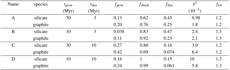
Table 3. Models with three free parameters.
Name species tgrow tdisr fgrow fshock fdisr δ2 ftot
(Myr) (Myr) (10−3)
A silicate 30 3 0.13 0.62 0.45 0.98 1.2
graphite 0.20 0.76 0.25 1.8 1.2
B silicate 10 3 0.038 0.83 0.47 2.4 1.3
graphite 0.11 0.92 0.23 2.1 1.3
C silicate 30 10 0.27 0.80 0.16 3.0 1.2
graphite 0.42 0.69 0.074 6.4 1.2
D silicate 10 10 0.16 1 0.15 10 1.3
graphite 0.24 0.99 0.061 5.8 1.3
fractions is unity: fgrow+fshock+fdisr=1. The results with
this fitting are shown in Table 2. The best-fitting values of
fdisrvary from those in Table 1 within a difference of 10%
except for Model B of silicate (25% less). However, the best-fitting values of fgrow is broadly 1/2–2/3 of those in
Table 1. As a result, Eq. (6) is not satisfied, and the total dust mass decreases.
Next, we perform fitting to the MRN size distribution with the parameters fgrow, fshock, and fdisr free. The
re-sults are shown in Table 3. Again, the values of fdisrdiffer
by only10% except for Model B of silicate (18% less). However, fgrow is only∼1/3–2/3 of the values in Table 1,
and fshock is made large to compensate for the decreased
fgrow. This means that the fitting is practically dominated by
the balance between the decreased small grains in shock de-struction and the increased small grains in disruption (shat-tering). Because of the dominance of fshock, Eq. (6) is not
satisfied, and the total dust mass decreases. 4.4 Extinction curve
Fig. 4. Upper panel: Extinction curves (extinction per hydrogen nucleus as a function of wavelength) calculated for the components used for the fitting to the grain size distribution. These components are shown in Fig. 1. The thin solid, dashed, and dot-dashed lines represent individual components processed for the following processes: disruption (shatter-ing) for 3 Myr in Panel (a) and for 10 Myr in Panel (b), growth for 10 Myr in Panel (a) and for 30 Myr in Panel (b), and shock, respectively. The thick solid line shows the extinction curve forng,s(a)/1.8 (divided
by 1.8 because the component “g,s” contains a grain mass 1.8 times as much as the MRN). The dotted line presents the extinction curve for the MRN size distribution. The points show the observed Milky Way ex-tinction curve taken from Pei (1992). Lower panel: Ratio of exex-tinction curves to the extinction curve of the MRN size distribution. The line species in the lower panel correspond to those in the upper panel.
function of wavelength and grain size is derived from the Mie theory, and is weighted for the grain size distribution per hydrogen nucleus to obtain the extinction curve per unit hydrogen nucleus (denoted asAλ/NH). The abundances of
silicate and graphite relative to hydrogen nuclei are already inherent in the models through the abundances of Si and C andξ (Section 2).
First, we show the extinction curves of the individual components, which are used to fit the MRN size distribu-tion, in Fig. 4. Grain growth does not make the extinction curve flatter in spite of the increase of the mean grain size. The reason is already explained in Hirashita (2012): accre-tion predominantly occurs at the smallest sizes. Since the extinction at short wavelengths is more sensitive to the
in-Fig. 5. Extinction curves (extinction per hydrogen nucleus as a function of wavelength) calculated for Models A–D (upper panel). The ratio to the extinction curve for the MRN size distribution is also shown (lower panel). The solid, thick dotted, dashed, and dot-dashed lines represent Models A, B, C, and D, respectively. The thin dotted line shows the extinction curve for the MRN size distribution. The points show the observed Milky Way extinction curve taken from Pei (1992).
Fig. 6. Same as Fig. 5 but we use the mean values between silicate and graphite for fgrowand fdisr.
crease of the mass of small grains than that at long wave-lengths, the extinction curve becomes rather steeper. Al-though coagulation flattens the extinction curve, the flatten-ing due to coagulation does not overwhelm the steepenflatten-ing due to the above effect of accretion.
Shock destruction makes the extinction curve flatter be-cause small grains are more easily destroyed than large grains. Grain disruption steepens the extinction curve be-cause of the production of a large number of small grains. The 0.22μm bump created by small graphite grains in this model becomes also prominent by grain disruption. We also show the extinction curve for the grain size distribu-tionng,s(a)(The componentng,s has a total dust mass 1.8
times as large as the initial value. To see the difference in the extinction curve, it would be helpful to make a compari-son under the same dust mass, song,s/1.8 is compared with
In Fig. 5, we show the extinction curves calculated for Models A–D. First of all, we confirm that the MRN size distribution reproduces the observed extinction curve (some small deviations can be fitted further if we adopt a more de-tailed functional form of the grain size distribution, which is beyond the scope of this paper; see Weingartner and Draine, 2001, for a detailed fitting). Comparing the extinction curve for the MRN size distribution and those for Models A–D, we observe that the extinction curve is reproduced within a difference of∼10%. Models A and C are successful, while Models B and D systematically underproduce the MRN ex-tinction curve (although the difference is small). The under-prediction by∼10% in Models B and D occurs because ftot
is∼0.9.
In the above, we adopted different values for fgrow and
fdisrbetween silicate and graphite. As mentioned in
Sub-section 2.2, if both species are well mixed in the ISM, they would have common values of these parameters. In Fig. 6, we show the extinction curve by taking the average of the values for silicate and graphite (for example, fgrow =0.35
and fdisr = 0.35 for Model A). We find that the
differ-ence between Figs. 5 and 6 is small. Therefore, the mean values work to reproduce the Milky Way extinction curves. The mean values are in the range of fgrow = 0.3–0.5 and
fdisr = 0.1–0.4. We conclude that the synthetic grain
size distributions with these parameter ranges reproduce the Milky Way extinction curve.
5.
Conclusion
In our previous papers (Nozawaet al., 2006; Hirashita and Yan, 2009; Hirashita, 2012), we showed that dust grains are quickly processed by shock destruction, disruption, and grain growth. In this paper, we have examined if the MRN grain size distribution, which is believed to represent the grain size distribution in the Milky Way, can be reproduced by the processed grain size distributions. We “synthesized” the grain size distribution by summing the processed grain size distributions under the condition that the decrease of dust mass by shock destruction is compensated by grain growth. We have found that the synthetic grain size distri-bution can reproduce the MRN grain size distridistri-bution in the sense that the deficiency of small grains by grain growth and shock destruction can be compensated by the production of small grains by disruption. The values of the fitting parame-ters indicate that, among the processed grains, 30–50% are growing in a dense medium, 20–40% are being destroyed by shocks in a diffuse medium, and 10–40% are being shat-tered in a diffuse medium (the percentage shows the relative importance of each process). The extinction curves calcu-lated by the synthesized grain size distributions reproduce the observed Milky Way extinction curve within a differ-ence of ∼10%. This means that our approach of synthe-sizing the grain size distribution based on major processing mechanisms (i.e., grain growth, shock destruction, and dis-ruption) is promising as a general method to “reconstruct” the extinction curve.
Acknowledgments. We are grateful to C. Wickramasinghe and an anonymous reviewer for helpful comments in their review of this paper. HH has been supported through NSC grant
99-2112-M-001-006-MY3. TN has been supported by a World Premier International Research Center Initiative (WPI Initiative), MEXT, Japan, and by the Grant-in-Aid for Scientific Research of the Japan Society for the Promotion of Science (20340038, 22684004, 23224004).
References
Asano, R. S., T. T. Takeuchi, H. Hirashita, and A. K. Inoue, Dust formation history of galaxies: A critical role of metallicity for the dust mass growth by accreting materials in the interstellar medium,Earth Planets Space, 65, this issue, 213–222, 2013.
Bianchi, S. and R. Schneider, Dust formation and survival in supernova ejecta,Mon. Not. R. Astron. Soc.,378, 973–982, 2007.
Bishop, J. E. L. and T. M. Searle, Power-law asymptotic mass distributions for systems of accreting or fragmenting bodies,Mon. Not. R. Astron. Soc.,203, 987–1009, 1983.
Calzetti, D., The dust opacity of star-forming galaxies,Publ. Astron. Soc. Pac.,113, 1449–1485, 2001.
Draine, B. T., Interstellar dust grains,Ann. Rev. Astron. Astrophys.,41, 241–289, 2003.
Draine, B. T., Interstellar dust models and evolutionary implications, in cosmic dust—near and far, inASP Conference Series 414, edited by Th. Henning, E. Gr¨un, and J. Steinacker, 453–472, Astromomical Society of the Pacific, San Francisco, 2009
Draine, B. T. and A. Li, Infrared emission from interstellar dust. I. Stochas-tic heating of small grains,Astrophys. J.,551, 807–824, 2001. Dwek, E., The evolution of the elemental abundances in the gas and dust
phases of the galaxy,Astrophys. J.,501, 643–665, 1998.
Gauger, A., Y. Y. Balega, P. Irrgang, R. Osterbart, and G. Weigelt, High-resolution speckle masking interferometry and radiative transfer model-ing of the oxygen-rich AGB star AFGL 2290,Astron. Astrophys.,346, 505–519, 1998.
Groenewegen, M. A. T., IRC +10 216 revisited. I. The circumstellar dust shell,Astron. Astrophys.,317, 503–520, 1997.
Hellyer, B., The fragmentation of the asteroids,Mon. Not. R. Astron. Soc., 148, 383–390, 1970.
Hirashita, H., Dust growth in the interstellar medium: How do accretion and coagulation interplay?,Mon. Not. R. Astron. Soc., 2012 (in press). Hirashita, H. and T.-M. Kuo, Effects of grain size distribution on the
interstellar dust mass growth,Mon. Not. R. Astron. Soc.,416, 1795– 1801, 2011.
Hirashita, H. and K. Omukai, Dust coagulation in star formation with different metallicities,Mon. Not. R. Astron. Soc.,399, 1795–1801, 2009. Hirashita, H. and H. Yan, Shattering and coagulation of dust grains in in-terstellar turbulence,Mon. Not. R. Astron. Soc.,394, 1061–1074, 2009. H¨ofner, S., Winds of M-type AGB stars driven by micron-sized grains,
Astron. Astrophys.,491, L1–L4, 2008.
Hoyle, F. and N. C. Wickramasinghe, Interstellar grains,Nature,223, 450– 462, 1969.
Hoyle, F. and N. C. Wickramasinghe,The Theory of Cosmic Grains, Kluwer Academic Publishers, Dordrecht, 1991.
Inoue, A. K., Evolution of dust-to-metal ratio in galaxies,Publ. Astron. Soc. Jpn.,55, 901–909, 2003.
Inoue, A. K., The origin of dust in galaxies,Earth Planets Space,63, 1027– 1039, 2011.
Jones, A., A. G. G. M. Tielens, and D. Hollenbach, Grain shattering in shocks: The interstellar grain size distribution,Astrophys. J.,469, 740– 764, 1996.
Kim, S.-H., P. G. Martin, and P. D. Hendry, The size distribution of inter-stellar dust particles as determined from extinction,Astrophys. J.,422, 164–175, 1994.
Lada, C. J., M. Lombardi, and J. F. Alves, On the star formation rates in molecular clouds,Astrophys. J.,724, 687–693, 2010.
Liffman, K. and D. D. Clayton, Stochastic evolution of refractory inter-stellar dust during the chemical evolution of a two-phase interinter-stellar medium,Astrophys. J.,340, 853–868, 1989.
Mathis, J. S., W. Rumpl, and K. H. Nordsieck, The size distribution of interstellar grains,Astrophys. J.,217, 425–433, 1977 (MRN). Mattsson, L. and S. H¨ofner, Dust-driven mass loss from carbon stars as a
function of stellar parameters. II. Effects of grain size on wind proper-ties,Astron. Astrophys.,533, A42, 2011.
McKee, C. F., Dust destruction in the interstellar medium, inInterstellar Dust, Proc. of IAU 135, edited by L. J. Allamandola and A. G. G. M. Tielens, 431–443, Kluwer, Dordrecht, 1989.
shocks driven by supernovae in the early universe,Astrophys. J.,648, 435–451, 2006.
Nozawa, T., T. Kozasa, A. Habe, E. Dwek, H. Umeda, N. Tominaga, K. Maeda, and K. Nomoto, Evolution of dust in primordial supernova remnants: Can dust grains formed in the ejecta survive and be injected into the early interstellar medium?,Astrophys. J.,666, 955–966, 2007. O’Donnell, J. E. and J. S. Mathis, Dust grain size distributions and the
abundance of refractory elements in the diffuse interstellar medium,
Astrophys. J.,479, 806–817, 1997.
Ormel, C. W., D. Paszun, C. Dominik, and A. G. G. M. Tielens, Dust co-agulation and fragmentation in molecular clouds. I. How collisions be-tween dust aggregates alter the dust size distribution,Astron. Astrophys., 502, 845–869, 2009.
Pei, Y. C., Interstellar dust from the Milky Way to the Magellanic Clouds,
Astrophys. J.,395, 130–139, 1992.
Savage, B. D. and K. R. Sembach, Interstellar abundances from absorption-line observations with the Hubble Space Telescope,Ann. Rev. Astron. Astrophys.,34, 279–330, 1996.
Weingartner, J. C. and B. T. Draine, Dust grain-size distributions and ex-tinction in the Milky Way, Large Magellanic Cloud, and Small Magel-lanic Cloud,Astrophys. J.,548, 296–309, 2001.
Wickramasinghe, N. C., Interstellar grains, inThe International Astro-physics Series, Chapman & Hall, London, 1967.
Yamasawa, D., A. Habe, T. Kozasa, T. Nozawa, H. Hirashita, H. Umeda, and K. Nomoto, The role of dust in the early universe. I. Protogalaxy evolution,Astrophys. J.,735, 44, 2011.
Yan, H., A. Lazarian, and B. T. Draine, Dust dynamics in compressible magnetohydrodynamic turbulence,Astrophys. J.,616, 895–911, 2004. Zhukovska, S., H.-P. Gail, and M. Trieloff, Evolution of interstellar dust
and stardust in the solar neighbourhood,Astron. Astrophys.,479, 453– 480, 2008.