R E S E A R C H
Open Access
A new blind algorithm for channel
estimation in OFDM-based
amplify-and-forward two-way relay networks
Tzu-Chiao Lin
*and See-May Phoong
Abstract
In this paper, we propose a blind channel estimation algorithm for the amplify-and-forward (AF) two-way relay network (TWRN) which consists of two terminal nodes and one relay node. The orthogonal frequency division multiplexing (OFDM) modulation is adopted for frequency selective channel. Both cyclic prefix (CP) and zero padding (ZP) are considered. The two cascaded channels are estimated in two steps. First, the cascaded channel causing the self-interference is estimated using a proposed power reduction method. Then, the other cascaded channel from source to destination is estimated by subspace method. Closed-form formulas for channel estimates are derived. In addition, we also carry out the theoretical mean square error analysis and derive the approximated Cramer-Rao bounds.
Keywords: Blind channel estimation, Orthogonal frequency division multiplexing (OFDM), Two-way relay network (TWRN)
1 Introduction
Research on wireless relay networks became popular since the pioneering work [1] developed low-complexity coop-erative diversity strategies. In [1], data streams flow uni-directionally from the source to the relay and then to the destination. This network structure is known as the one-way relay network (OWRN). However, since most communication systems are bidirectional, it is necessary to consider the situation when the source node and the destination node exchange their roles. Such a relay net-work is known as the two-way relay netnet-work (TWRN). In TWRN, the relay treats the received signals in a “network coding”-like manner [2], and the terminals can recover the signal collision since they know their own transmitted sig-nals. As a result, the overall communication rate between two source terminals in TWRN is approximately twice that achieved in OWRN [3].
Despite its throughput advantage, TWRN faces more challenges in terms of transceiver design, relay processing optimization, and transmission protocol development. In
*Correspondence:[email protected]
Graduate Institute of Communication Engineering and Department of EE, National Taiwan University, Taipei, Taiwan
[4], the capacity analysis and the achievable rate region for amplify-and-forward (AF) and decode-and-forward (DF) TWRN are explored. In [5], the authors point out that the throughput of AF-TWRN is 1.5 times of DF-TWRN. The distributed space-time code (STC) at relays for both AF-TWRN and DF-TWRN has been developed in [6]. Moreover, the optimal beamforming with full channel knowledge at the multi-antenna relay that maximizes the overall system capacity of AF-TWRN is derived in [7]. In [8], the authors address the problem of robust linear relay precoder and destination equalizer design for multiple-input multiple-output relay systems. In [9], the authors compare several network-coding AF-TWRN and consider imperfect time synchronization. Most existing works on TWRN [2–9] have assumed perfect channel state infor-mation (CSI) at the relay node and/or the source termi-nals. While traditional channel estimation methods can be applied to DF-TWRN, the channel estimation problem for AF-TWRN is more challenging due to the self-interfering signals.
In traditional channel estimation methods for point-to-point systems, they can be divided into two groups: data-aided (DA) [10–17] and non data-aided (blind) [18–26]. In general, DA channel estimation methods differ in the
way they interpolate or filter punctual DA least square (DA-LS) channel estimates over data subcarriers. This can be accomplished using time-frequency Wiener filtering [10,11], which is optimal in the minimum mean square error (MMSE) sense if knowledge of the channel statistics (KCS) is available. On the other hand, channel estima-tion can be accomplished by elaborating raw estimates in the time domain using a discrete Fourier transform (DFT)-based scheme. In [12], the MMSE channel estima-tor working in the time domain has been proposed. In order to reduce computational complexity, using the sin-gular value decomposition and several low-rank approxi-mations to the MMSE estimator has been proposed in [13] and [14]. Li et al. [12–14] also require complete KCS. In [15], the authors compare the MMSE approach with maxi-mum likelihood (ML) channel estimation, where complete KCS is not required. This latter approach works well with dense multipath channels and quasi-uniform profiles. In practice, after the inverse DFT (IDFT), not all the channel impulse response (CIR) samples are significant because many may correspond to delays where no propagation channel paths are actually present. Therefore, the authors in [16] exploit this idea to estimate channel. In [17], the authors propose a method to approach the MMSE chan-nel estimation performance, while avoiding the need for a priori KCS.
For blind channel estimation methods, earlier works require either higher order statistics (HOS) of the received data [18] or over-sampling at the receiver [19]. By exploit-ing linear redundant precodexploit-ing , only second-order statis-tics (SOS) of the received data is required and these methods are robust to channel order overestimation [20,21]. Another popular blind algorithm is the so-called subspace-based algorithm which was originally developed in [19]. The subspace method has simple structure and achieves good performance. In [22], a blind channel iden-tification method by exploiting virtual carriers (VC) is derived. In [23], a generalization in cyclic prefix (CP) sys-tems is proposed. By arranging the received data appro-priately, [23] generates a rank-deduction matrix, and thus, subspace method can work. In [24], the authors propose another simpler arrangement of the received data. Pan and Phoong [25] and [26] utilize the repetition method to reduce the number of required received data and consider the existence of VCs.
As in the traditional point-to-point systems, study of channel estimation algorithm is also demanded for AF-TWRN systems [27–34]. DA channel estimation methods for AF-TWRN are proposed in [27–30]. Gao et al. [27] develops an optimal training design for flat-fading envi-ronment. The authors also combine their algorithm with orthogonal frequency division multiplexing (OFDM) to estimate the channel impulse responses for frequency selective environment in [28]. The case of multiple-input
multiple-output is considered in [29], and [30] provides two channel training algorithms for channel estimation.
On the other hand, [31–34] are blind channel esti-mation methods. In [31], the authors propose a ML approach to estimate the flat-fading channels blindly, but the transmitted signals are limited to constant modulus modulation. Zhao et al. [32] find a closed-form solution and thus provides a low-complexity ML algorithm. For non-constant modulus modulation, [33] gives an iterative algorithm, which is based on the maximum a posteri-ori (MAP) approach, and it requires a large number of received blocks. In [34], the authors consider the fre-quency selective environment. They apply a non-unitary linear precoding at both terminals and derive a blind channel estimation algorithm from SOS of the received signals. However, the use of non-unitary linear precoding leads to degradation in bit error rate (BER) performance.
In this paper, we develop a blind channel estimation algorithm for AF-TWRN under OFDM modulation. Our method consists of two steps. The first step is to esti-mate the cascaded channel causing the self-interference. Since the terminal knows its own transmitted signal, we choose the method based on power reduction to estimate the channel, which is also named LS method. The self-interference signal can be removed by using the estimated channel. The second step is to estimate the cascaded channel from source to destination. We utilize the rank reduction method, which is also known as subspace-based algorithm [23–26]. This is because subspace methods do not require complete KCS, work well with all mul-tipath channels, and achieve good performance. Closed-form Closed-formulas for these two cascaded channel estimates are derived. The theoretical performance analysis and approximated Cramer-Rao bounds (ACRB) are given as well. The proposed method can be applied to both CP-based and zero padding (ZP)-CP-based OFDM systems. Sim-ulation results will be provided to show the performance of the proposed method.
The rest of this paper is organized as follows. The sys-tem model for CP-OFDM AF-TWRN is introduced in Section2. Section3describes the proposed algorithm for blind channel estimation. In Section 4, we analyze the performance of the proposed channel estimation meth-ods and the ACRBs. Simulation results are presented in Section5, and concluding remarks are made in Section6. The results in Section 3.1 and 3.2 of this paper have appeared in a conference paper [35].
Notation In this paper, E{x} stands for the statistical expectation of the random variable x. The symbolsAT, A∗, andA†denote the transpose, the complex conjugate, and the conjugate-transpose of matrix A, respectively. AFis the Frobenius norm of matrixA. IfAis a square,
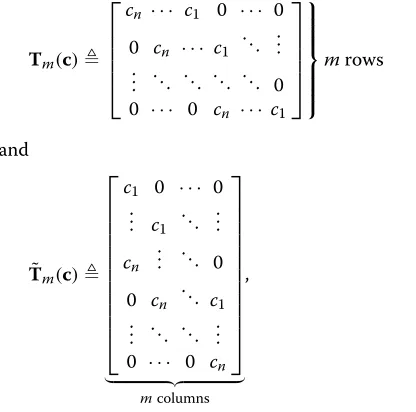
identity matrix, whereas0represents an all-zero matrix with appropriate dimension. j = √−1 is the imagi-nary unit. Tm(c) and T˜m(c) are two Toeplitz matrices
Consider a TWRN with two terminal nodesT1andT2, and one relay nodeR, as shown in Fig.1. Each node has one antenna which cannot transmit and receive simulta-neously. The channel from Ti to R is denoted as fi = [fi,0,fi,1,. . .,fi,L]T, whereas the one fromRback toTi is denoted asgi =
gi,0,gi,1,. . .,gi,LT fori = 1 and 2. For notational simplicity, we assume that the lengths off1,f2, g1, andg2do not exceedL+1.1Similar to most other algo-rithms, we assume that the channels do not change when the channel estimation is performed.
2.1 OFDM modulation at terminals
Denote the kth OFDM block from Ti as s(ki) =
sk(i,0),sk(i,1),. . .,s(ki,)N−1 T
, where N is the OFDM block length. The corresponding time domain signal block is obtained from the normalized IDFT as
x(ki)=W†s(ki)=
xk(i,0) xk(i,1) · · · x(ki,)N−1 T
, (3)
whereWis theN×Nnormalized DFT matrix with the
(m,n)th entry given by √1
Ne
−j2πmn/N. To maintain the subcarrier orthogonality during the overall transmission, we propose to add a CP of length 2L.2 This implicitly requiresN ≥ 2Lwhich is nevertheless satisfied by most OFDM systems. Define x(ki,)cp =[x(ki,)N−2L,. . .,x(ki,)N−1]T. The signal sent out fromTiis expressed as
x(ki,)cpT x(ki)TT fori=1 and 2.
2.2 Relay processing
The relayRreceives the signal [34]
rk =
Moreover, each element in the noise vector nk,r is assumed to be independent and identically distributed (i.i.d.) zero-mean complex white Gaussian.
We assume that the relayRemploys the amplify-and-forward scheme. It scalesrkby the factor of
α=
wherePr is the average transmission power ofR. In the second equality, we have made the assumptions that the transmitted signalsx(k1),xk(2), and the received noisenk,r are uncorrelated with variancesσ12,σ22, and σ2
nr,
respec-tively. Then, the relay broadcastsαrkto both terminals.
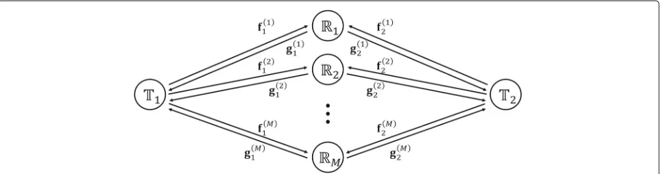
Fig. 1System configuration for two-way relay network. It shows a two-way relay network with two terminal nodesT1andT2, and one relay node R. Each node has one antenna which cannot transmit and receive simultaneously. The channel fromTitoRis denoted asfi, whereas the one from
2.3 Signal reformulation at terminals
Due to symmetry, we only illustrate the processing atT1. The(N+2L)×1 vector received atT1can be expressed as
and each element in the noise vectornk,t is assumed to be i.i.d. zero-mean complex white Gaussian, with variance
σ2 linear convolution between two vectors by the fact that the multiplication of two Toeplitz matrices is still a Toeplitz matrix. The last termnk,edenotes the equivalent noise
nk,e=αTN+2L(g1)
2.4 Data detection at terminals
After removing the first 2Lelements ofykin (9), we obtain can be efficiently performed using fast Fourier transform. SoT1can recover the data fromT2if bothh1andh2are available. Hence, our goal is to estimateh1andh2. Below, we will show how to blindly estimate these two cascaded channels from the received signalyk.
3 Proposed method for channel estimation In this paper, we assume that x(k1) andx(k2) are uncorre-lated. Moreover, the transmitted signals and the noises are uncorrelated as well. Under these two assumptions, we propose an algorithm to estimate h1 andh2blindly. Though our derivations are based on CP-OFDM system, the results can be also extended to ZP-OFDM system. The details will be discussed later.
3.1 The estimation ofh1
Let us look at the received vectory¯k in (11). Notice that x(k1)is known atT1. If we have a perfect estimate ofh1, then the first term at the right-hand side of (11) can be eliminated completely from y¯k. Due to uncorrelatedness ofx(k1),xk(2), andn¯k,e, the power ofy¯kwill be reduced when x(k1)is eliminated fromy¯k. Based on this power reduction, we are able to derive a closed-form formula for an estimate of the(2L+1)×1 vectorh1, as shown below.
Define a cost function
¯
is a diagonal matrix with the elements of s(k1)on the main diagonal, andW2L+1is the first 2L+1 columns of the DFT matrixW. Let
y=y¯T0 y¯1T · · · ¯yTK−1T (16) where the symbol⊗denotes the Kronecker product. The least squares solution of (18) can be calculated as
ˆ lation symbols are statistically independent. In this case, (19) can be approximated as
ˆ
where the symbol denotes the Hadamard product. Notice that there is no scalar ambiguity in the estimation ofh1sincesk(1)andy¯kare known atT1.
3.2 The estimation ofh2
In order to estimate the (2L + 1) × 1 vector h2, we first remove the self-interfering signal from the received vector. Define
Note that the vectorzk is simply the received vector in a usual CP-OFDM system with channelh2and transmit-ted vectorx(k2). Many blind estimation methods have been proposed for the estimation ofh2fromzk. Below, we will adopt the subspace-based algorithm in [24]. Define the re-modulated vector entries ofzk. Next, we construct the vector
vk =zk− ˜zk. (24)
Carrying out the whitening process onvk, we get the whitened vectorv(kw)=R−w1/2vkand its covariance matrix
is that T1 collects K ≥ N blocks. Utilizing eigenvalue decomposition, (27) can be computed as
R(vw)=UsU†s +σn2eUoU
†
o, (28)
whereis anN×Ndiagonal matrix and the(N+2L)×N
matrixUs spans the signal subspace. On the other hand, the (N +2L)×2LmatrixUo spans the noise subspace. That is,
Uo†R−w1/2T˜N(h2)=0. (29) Let
Ji=
⎡
⎣ 0i×I2(L2+L+11) 0(N−1−i)×(2L+1)
⎤
⎦ fori=0, 1,. . .,N−1.
(30) Then, (29) can be rewritten as
⎡ ⎢ ⎢ ⎣
U†
oR
−1/2
w J0 .. . U†oR−w1/2JN−1
⎤ ⎥ ⎥ ⎦
U
h2=0. (31)
Hence, we can estimateh2(up to a scalar ambiguity) by calculating the eigenvector corresponding to the smallest eigenvalue ofU†U.
In summary, our algorithm is as follows.
1. Estimateh1by (20).
2. Eliminate the interference fromT1by (21).
3. Calculatev(kw)=Rw−1/2vkby (24) and (26) and obtain
the(N+2L)×2LmatrixUospanning the noise
subspace by eigenvalue decomposition.
4. Estimateh2(up to a scalar ambiguity) by calculating
the eigenvector corresponding to the smallest eigenvalue ofU†U.
3.3 A note on the identifiability issue
Note that the estimate of h1 is unique because the cost function in (14) has a unique minimum athˆ1 = h1. The second channelh2is estimated by the subspace method. Let us look at the vector zk in (22). When the self-interfering signal is completely eliminated, the remaining partzkis identical to the case of single-input single-output (SISO) CP-OFDM system in [24]. The identifiability issue of this method has been studied in [24]. It has been shown that ifh2,0=0, then the vectorh2is uniquely determined (up to a scalar ambiguity).
3.4 Comparison with an existing work
A blind channel estimation algorithm in OFDM-based TWRN was proposed in [34]. Comparing our method with that in [34], there are two major differences. One is that [34] requires a precoding matrixP, where
PP†=
⎡ ⎢ ⎢ ⎢ ⎢ ⎣
1 θ · · · θ
θ 1 . .. ... ..
. . .. ... θ
θ · · · θ 1
⎤ ⎥ ⎥ ⎥ ⎥ ⎦.
A necessary condition onθ is−N1−1 ≤θ ≤ 1. In other words, thekth transmitted vector fromTiis the precoded vectorPs(ki)instead ofsk(i). Notice that forθ =0,Pis not a unitary matrix. The channel noise can be amplified when the receiver performs the operationP−1. It was shown in [34] that whenθ increases from 0 to 1, the mean square error (MSE) of channel estimate decreases. Due to noise amplification, larger θ does not necessarily yield smaller BER, so there exists a compromise between channel esti-mation error and BER. Another difference between our method and [34] is that there is a 2×2 ambiguity matrix in [34], or equivalently, there are four ambiguity scalars. On the other hand, there is only one ambiguity scalar in our algorithm. In terms of complexity, we can see that the main complexity of our method is the computation of the eigenvalue decomposition of anN×N matrix in (28), whereas the eigenvalue decomposition in [34] is for a(2L+1)×(2L+1)matrix. Hence, our method is more complicated than [34].
3.5 Repeated use of the remodulated vectorvk
To obtain Uo in (28), T1 has to collectK ≥ N blocks. In OFDM systems, N is usually large. The number of blocks,K, needed for the channel estimation is large. In order to reduce the required block numberK, we can use the repetition method proposed in [23, 25, 26]. Define the repetition parameterQand form the matrixT˜Q(vk), wherevkis defined in (24). According to (25),T˜Q(vk)can be represented as
˜
TQ(vk)= ˜TN+Q−1(h2)T˜Q(dk)+ ˜TQ(ηk). (32) It was shown in [25] thatT˜Q(ηk)is colored noise, and its covariance matrix can be calculated as
E #
˜
TQ .
ηk /˜
T†Q(ηk)
$
=σ2
ne
Q
q=1
⎡ ⎢ ⎣
0(q−1)×(q−1) 0 0
0 Rw 0
0 0 0(Q−q)×(Q−q) ⎤ ⎥ ⎦
=σ2
neEE †,
(33) where we have applied the eigenvalue decomposition in the second equality. Therefore, we need to whiten the matrix T˜Q(vk) by E−1/2E†. Since each vector vk is repeatedQtimes in (32), the required number of blocks becomes K ≥ NQ−1 + 1 blocks [23]. Collecting these
3.6 Multiple relay nodes
The extension to the case of multiple relay nodes is straight forward as shown in Fig.2. Suppose that we have
Mrelay nodesR1,R2,. . .,RM. Let the channels fromTito
Rmbe denoted asf(im)and the channels fromRmtoTibe denoted asg(im). Then, (4) becomes
r(km)= 2
i=1 TN+2L
f(im)
⎡⎢ ⎣
x(ki−)1,isi x(ki,)cp x(ki)
⎤ ⎥
⎦+n(km,r), (34)
where r(km) is the signal received by relay nodeRm and n(km,r)is the noise atRm. WhenT1receives the signal, (7) becomes
yk = M
m=1 TN+2L
g(1m) αmr (m) k−1,isi
αmr(km)
+nk,t, (35)
where αm is the amplification scalar in the relay node
Rm. Combining (34) with (35), the received vector atT1 continues to have the form given in (9), but now the cascaded channels areh1 = 0Mm=1αm
g(1m)∗f(1m)and h2 = 0Mm=1αm
g(1m)∗f(2m)
, and the equivalent noise nk,ebecomes
nk,e= M
m=1
αmTN+2L
g(1m)
⎡ ⎢ ⎢ ⎢ ⎢ ⎣
n(km−)1,r(N+L)
.. .
n(km−)1,r(N+2L−1) n(km,r)
⎤ ⎥ ⎥ ⎥ ⎥ ⎦+nk,t.
Hence, the above methods can be applied to the case of multiple relay nodes.
3.7 The case of ZP-OFDM systems
The proposed method can be also applied to TWRN ZP-OFDM system. In this case, 2Lzeros are padded at the end ofx(ki)in (3) instead of adding the cyclic prefix of length
2L. Due to the padded zeros, the received vector does not suffer from ISI. Therefore, (9) can be rewritten as
yk = ˜TN(h1)x(k1)+ ˜TN(h2)x(k2)+nk,e. (36) To estimateh1, we modify the cost function in (12) as
J
ˆ h1
=E
1! !!yk− ˜TN
ˆ h1
x(k1)!!!2 F
2
. (37)
Following a procedure similar to (12)–(20), an estimate ofh1can be obtained by
ˆ h1=
1 N
√
N+2LKσ
2 1 ˜ W†2L+1
K−1
k=0
˜ WNx(k1)
∗
˜ Wyk
, (38)
whereW˜ is the(N+2L)×(N+2L)normalized DFT matrix with the (m,n)th entry given by √ 1
N+2Le
−j2πmn/(N+2L), whereasW˜2L+1andW˜N are respectively the first 2L+1 andNcolumns ofW.˜
Assume that the estimation ofh1is perfect so that we can eliminate the interference from T1. Similar to (21), define
zk =yk− ˜TN
ˆ h1
x(k1). (39)
Substituting (36) into (39), we have
zk = ˜TN(h2)xk(2)+nk,e. (40) This form is similar to (25), so we can follow the proce-dure in (25)–(31) to estimateh2. Note that the noisenk,eis (almost) white. Similar to the previous discussion, a nec-essary condition isK ≥ N. To reduce the limitation of a largeK, we exploit the repetition method in [26]. That is, we utilizeT˜Q(zk)instead ofzkto estimateh2, and the nec-essary condition becomesK ≥ NQ−1+1. In this case, the noise termT˜Q(nk,e)is colored (thoughnk,eis white) and the covariance matrix is [26]
E#T˜Q
Following a procedure similar to Section 3.5, one can obtain a blind estimate ofh2(up to a scalar ambiguity).
4 Analysis of MSE performance and Cramer-Rao bound
In this section, we will derive the theoretical MSE about channel estimation forh1andh2respectively. In the fol-lowing analysis, we assume that the channel taps are uncorrelated and the transmitted vectors x(ki) are also uncorrelated for differentkori.
4.1 The analysis ofh1estimate
In the estimation ofh1, we regard the signal fromT2as interference. Since (20) is the least squares solution of (18), the difference betweenhˆ1andh1can be calculated as
h1hˆ1−h1
whereξk denotes the interference and noise. From (11), we have
as its first column. Assuming that x(k2)andnk,eare uncorrelated, the covariance matrix ofξk can be computed as
E#ξkξ†k$=σ22C(h2)C†(h2)+σn2eIN
is theN×Ndiagonal matrix with diagonal entries from theN×1 frequency response vectorh2,f =
√ theoretical MSE can be calculated as
E h12F=trR h1
is the sum of the diagonal elements of R h1. Define the signal-to-noise ratio (SNR) as
SNR σ
where the second equality is obtained by using (10). Then, (45) can be written as Note from the above equation that the MSE is propor-tional to the signal power fromT2but inversely propor-tional to the signal power fromT1and the number of the received signal blocks. Moreover, for high SNR, the MSE floors at the value of 2NKL+1σ22
σ2 1h2
2
F.
4.2 The analysis ofh2estimate
During the estimation ofh2in Section3.2, it is assumed that the estimate ofh1is perfect. However, the estimation error h1will affect the accuracy of the estimation ofh2. From (21), if h1 = 0, the interference and noise terms can be written as
TN+2L( h1)
Letλ1 ≤ λ2 ≤ · · · ≤ λN+2L be the eigenvalues ofR(vw). The noise subspace Uo is the eigenspace corresponding to the smallest 2Leigenvalues λ1,λ2,. . .,λ2L. The error vectorζk can cause two effects: (i) it perturbs the noise subspaceUo and (ii) it also perturbs the eigenvalues, i.e.,
λ1+ λ1,λ2+ λ2,. . .,λN+2L+ λN+2L. Note thatλ2L belongs to the noise subspaceUoandλ2L+1belongs to the signal subspaceUs. Their differenceλ2L+1−λ2Lis usually large. Nevertheless, the perturbation on eigenvalues may lead to the caseλ2L+ λ2L> λ2L+1+ λ2L+1, especially when the SNR is low. In this case, the noise subspace will be polluted by the signal subspace and this will cause a large error in the estimation ofh2. Below, we derive the MSE by studying the following two cases separately.
Case I: λ2L+ λ2L< λ2L+1+ λ2L+1
In this case, we can exploit the first-order approximation of the perturbation to Uo. In [24], the channel estima-tion error has been derived. However, the theoretical MSE derived in [24] is based on white noise. As the noiseζkis colored, the formula derived in [24] is not applicable. For the case of colored noiseζk, we have derived a new for-mula and the theoretical MSE of theh2estimate can be calculated as covariance matrix ofζkand it can be written as
Rζ =2σ12R−w1/2E
In this case, our algorithm cannot find the accurate noise subspaceUobecause it has been polluted by signal subspaceUs. Thus, we assume that the eigenvector ofU corresponding to the smallest eigenvalue is random and uncorrelated to the true cascaded channelh2. Define this unit-norm eigenvector ash˜2. The scalar ambiguity can be calculated asα=h˜†2h2 estimate can be calculated as
E h22F=h†2E
Since the unit-norm vectorh˜2is assumed to be random, E#h˜2h˜†2
Overall MSE: Utilizing Bayes’ theorem, the theoretical MSE of theh2estimate can be written as
E h22F=PerrE
The derivation ofPerris given in AppendixA. Substitut-ing (50) and (55) into (56), the theoretical MSE of theh2 estimate can be represented as
E h22F
4.3 Approximated Cramer-Rao bound
we have σξ2 = σ22h22F +σn2e. Therefore, (59) can be simplified as
ACRB1= 2L+1
NK σ2
2h22F+σn2e σ2
1
. (60)
Notice that this form is the same as (45).
Next, we consider the ACRB ofh2. In [24], the authors have derived an ACRB and concluded that the ACRB is the same as the channel estimation MSE. Hence, from (50), an ACRB ofh2estimation is
ACRB2= 1 2Kσ22tr
1
UIN⊗U†oRζUo U†
2 . (61)
In the derivations of the ACRBs, the noises are assumed to be white even though they are actually colored. There-fore, the ACRBs in (60) and (61) are in general larger than or equal to the true Cramer-Rao bounds.
5 Simulation results
In the simulation, we consider a TWRN with one relay node. The channel tapsfi,landgi,lare generated as inde-pendent and identically distributed zero-mean complex Gaussian random variables with variances equal to 1/9. The order of these channels is L = 8, so the order of the cascaded channels is 2L= 16. The channels are nor-malized so thatf12F = f22F = g12F = g22F = 1. The channel does not change while the channel estima-tion is performed. The channel noise is additive white
Gaussian noise (AWGN), and the transmission symbols are 16-QAM with gray code. The size of the DFT matrix isN = 64, and the length of CP is 2L = 16. In all plots, we setσ12=σ22andσn2r =σn2t. The SNR is defined in (46), and the normalized MSE is defined as
1
Mc 0Mc
m=1
ˆh(im)−hi2F
hi2F fori=1 and 2,
where hˆ(im) represents the estimatedhi in themth trial.
Mc = 2000 denotes the total number of Monte-Carlo trials.
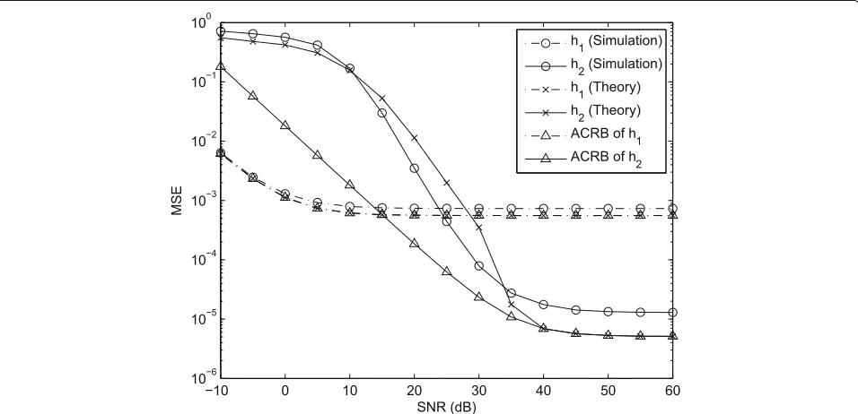
First, we look at the MSE performance of the proposed methods. The number of received blocks isK = 500. In Fig.3, we plot the normalized MSEs forh1andh2. The “simulation” curves ofh1andh2are obtained by (20) and (31), respectively, whereas the “theory” curves ofh1and h2are calculated by (47) and (58), respectively. Moreover, we also display the ACRBs ofh1andh2according to (60) and (61). From Fig.3, it can be seen that the simulated result, the theoretical MSE, and the ACRB ofh1is close. Moreover, the proposed method can give a good estimate of h1, even at very low SNR of 0 dB. One can see that the MSE floors at 2NKL+1 = 5.3×10⁻⁴at high SNR, and this confirms our analysis in (47). Forh2, the MSE perfor-mance is worse than that ofh1for SNR< 25 dB, but the MSE ofh2floors at a much smaller value of 1.2×10⁻⁵. This flooring happens at very high SNR, and the estima-tion error ofh1 affects the accuracy ofh2estimate. The
gap between numerical and theoretical results is small at high SNR. At low SNR, the gap between simulation result and ACRB becomes very large, but the theoretical curve is still close to the numerical curve. Recall that the theoretical MSE value is a combination of two cases in Section4.2, and the ACRB ofh2in (61) is equal to the the-oretical MSE when we do not consider the perturbation on eigenvalues, i.e., case II in Section4.2(case II usually happens at low SNR). Therefore, the difference between the theoretical MSE and ACRB ofh2at low SNR is caused by the perturbation of eigenvalues. From Fig.3, we con-clude that the change of eigenvalue sequence dominates the performance degradation at low SNR. In addition, the assumption of white noise in the derivation of ACRB also affects the accuracy, especially when the SNR is low.
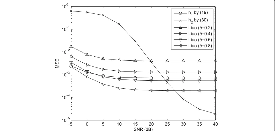
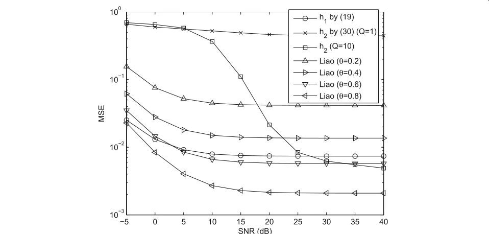
Next, we compare the performances of our method with the method proposed by Liao et al. in [34]. As men-tioned in Section3.4, Liao’s algorithm has a compromise between channel estimation error and BER. The param-eterθ in Liao’s algorithm is set to 0.2, 0.4, 0.6, and 0.8. From [34], it is found that θ = 0.4 yields a good BER performance when SNR = 25 dB. In Figs. 4 and5, the number of received blocks isK = 500. Figure4 shows the MSE performances. Since the MSEs ofh1andh2by Liao’s algorithm are the same, we plot one MSE curve only. From the figure, we see that as θ increases from 0.2 to 0.8, the MSE of Liao’s algorithm decreases. For the esti-mation ofh1, our method is better than Liao’s methods forθ = 0.2 and 0.4, but worse than that forθ = 0.6 and
θ = 0.8. As we will see in Fig.5, the BER performance
forθ = 0.8 is not good due to severe noise amplifica-tion. Forh2, Liao’s method is better at low SNR whereas our method is better at high SNR. In Fig. 5, we show BER performances. Zero-forcing equalizers are used at the receiver. The “perfect compensation” represents the case that the channel taps are perfectly known at the receiver. It is seen that among the four curves ofθ = 0.2, 0.4, 0.6, 0.8, Liao’s method has the best BER performance whenθ is set as 0.4 for SNR = 25 dB. Though the MSE of Liao’s method is the smallest when θ = 0.8, its BER perfor-mance is not good due to the noise amplification problem of the precoding matrix. These results are matched with [34]. From Fig. 5, we see that the proposed algorithm outperforms Liao’s methods when SNR ≥ 15 dB, and the performance of our method is close to the perfect compensation.
Figures 6and7 show the simulation results when the number of blocks isK = 50. In this case,K < N, and thus, the estimation of h2 by (31) does not work. We exploit the repetition method discussed in Section3.5to solve this issue. We set the repetition parameterQ= 10, and the necessary conditionK ≥ NQ−1+1 is satisfied. In Fig.6, the MSE performance is shown. We can observe that the repetition method is extremely useful when the terminal receives few blocks. On the other hand,h1 esti-mation by (20) and Liao’s algorithm are based on the power reduction, so there is no limitation on the num-ber of blocksK. From the figure, we see that the proposed method outperforms Liao’s algorithms withθ = 0.2 and 0.4 for all SNR. In Fig.7, the performance is measured by
Fig. 5Comparison of the BER forK=500. We compare the BER performances of our method with the method proposed by Liao et al. in [34]. The parameterθin Liao’s algorithm is set to 0.2, 0.4, 0.6, and 0.8. The number of received blocks isK=500
BER. It can be seen that the proposed algorithm performs better than Liao’s method when SNR ≥ 15 dB. Compar-ing Fig.7with Fig.5, we find that the BER performance degrades when K reduces from 500 to 50. This is due to the larger channel estimation errors for K = 50 and imperfect interference cancelation byh1using (21).
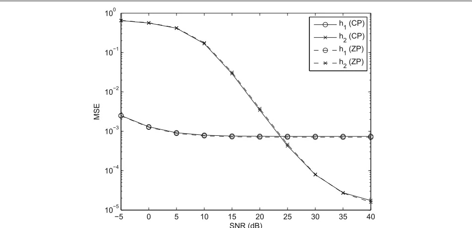
Finally, we compare the proposed algorithm for CP-OFDM and ZP-CP-OFDM systems. In Fig.8, the solid curves and the dashed curves represent the MSEs for CP-OFDM and ZP-OFDM, respectively. We can find that the perfor-mances are almost the same. In other words, our method works well for both CP and ZP systems.
Fig. 7Comparison of the BER forK=50. We compare the BER performances of our method with the method proposed by Liao et al. in [34]. The parameterθin Liao’s algorithm is set to 0.2, 0.4, 0.6, and 0.8. The number of received blocks isK=50
6 Conclusions
In this paper, we propose a blind channel estimation method in OFDM-based amplify-and-forward two-way relay networks. The first cascaded channelh1is estimated by the power reduction method whereas the second cas-caded channel h2 is estimated by the subspace method.
Close-form formulas are derived. We also analyze the theoretical performance and derive the ACRBs for chan-nel estimation. Our algorithm can be applied to both CP-OFDM and ZP-OFDM systems, and it can use repe-tition method to handle the case of few received blocks. Simulation results verify our analysis.
Endnotes
1The proposed method can be applied to the more
gen-eral case of different channel lengths by simply using an appropriate cyclic prefix length.
2IfT
1andT2add CP of lengthL, then the relay needs to carry out the operations of OFDM symbol timing syn-chronization, CP removal, and CP insertion. In order to simplify the tasks of the relay,T1andT2add CP of length 2L.
Appendix A
A proof of (57)
To simplify our derivation, we utilize the fact that this condition usually occurs at low SNR. From (47) and the simulation in Section5, it can be seen that the estimate of h1is still quite accurate at low SNR, so the second term nk,e in (48) is dominant. Let λ1 ≤ λ2 ≤ · · · ≤ λN+2L be the eigenvalues of R(vw) and the corresponding unit-norm eigenvectors are respectively b1,b2,. . .,bN+2L. By
Since the received signals are finite and the second term in (48) is dominant, we have the following approximation:
1 matrix with mean0. For largeK, the central limit theorem indicates that the diagonal entries of N are real normal distributed and the other entries are circularly symmetric complex normal distributed [37]. According to the result in [38], all entries ofNhave the same variance K1σ4
ne.
From matrix theory [39], the eigenvalue perturbation
λican be approximated asb†iNbi. Then, the mean is
and the variance is
E| λi|2=E
function. Thus, (65) can be rewritten as
E| λi|2
Notice thatNis normal distributed andbi is constant, so the random variable λiis normal distributed as well. It means that the probability of λ2L + λ2L ≥ λ2L+1+
ACRB: Approximated cramer-rao bound; AF: Amplify-and-forward; AWGN: Additive white Gaussian noise; BER: Bit error rate; CIR: Channel impulse response; CP: Cyclic prefix; CSI: Channel state information; DA: Data-aided; DF: Decode-and-forward; DFT: Discrete fourier transform; HOS: Higher order statistics; IDFT: Inverse discrete fourier transform; i.i.d.: Independent and identically distributed; ISI: Inter-symbol interference; KCS: Knowledge of the channel statistics; LS: Least squares; MAP: Maximum a posteriori; ML: Maximum likelihood; MMSE: Minimum mean square error; MSE: Mean square error; OFDM: Orthogonal frequency division multiplexing; OWRN: One-way relay network; SISO: Single-input single-output; SNR: Signal-to-noise ratio; SOS: Second-order statistics; STC: Space-time code; TWRN: Two-way relay network; VC: Virtual carrier; ZP: Zero padding
Funding
This work was supported by the Ministry of Science and Technology, Taiwan, R.O.C., under grant no. 106-2221-E-002-033.
Authors’ contributions
T-CL and S-MP constructed the theory. T-CL performed simulations and wrote a draft. S-MP modified the paper. Both authors read and approved the final manuscript.
Competing interests
The authors declare that they have no competing interests.
Publisher’s Note
Received: 14 July 2017 Accepted: 26 June 2018
References
1. JN Laneman, DNC Tse, GW Wornell, Cooperative diversity in wireless networks: efficient protocols and outage behavior. IEEE Trans. Inf. Theory.
50(12), 3062–3080 (2004)
2. S Katti, S Gollakota, D Katabi, Embracing wireless interference: analog network coding. Comput. Sci. Artif. Intell. Lab. Tech. Rep (2007) 3. B Rankov, A Wittneben, Spectral efficient signaling for half-duplex relay
channels. Annual Conference on Signals, Systems, and Computers, 1066–1071 (2005)
4. B Rankov, A Wittneben, Achievable rate regions for the two-way relay channel. International Symposium on Information Theory (ISIT), 1668–1672 (2006)
5. P Popovski, H Yomo, Wireless network coding by amplify-and-forward for bi-directional traffic flows. IEEE Commun. Lett.11(1), 16–18 (2007) 6. T Cui, F Gao, T Ho, A Nallanathan, Distributed space-time coding for
two-way wireless relay networks. International Conference on Communications (ICC), 3888–3892 (2008)
7. R Zhang, Y-C Liang, CC Chai, S Cui, Optimal beamforming for two-way multi-antenna relay channel with analogue network coding. IEEE J. Sel. Areas Commun.27(5), 699–712 (2009)
8. C Xing, S Ma, Y-C Wu, Robust joint design of linear relay precoder and destination equalizer for dual-hop amplify-and-forward MIMO relay systems. IEEE Trans. Signal Process.58(4), 2273–2283 (2010) 9. MW Baidas, AB MacKenzie, RM Buehrer, Network-coded bi-directional
relaying for amplify-and-forward cooperative networks: a comparative study. IEEE Trans. Wirel. Commun.12(7), 3238–3252 (2013)
10. P Hoeher, S Kaiser, P Robertson, Two-dimensional pilot symbol aided channel estimation by Wiener filtering. IEEE Int. Conf. Acoust. Speech Signal Process. (ICASSP).3, 1845–1848 (1997)
11. P Hoeher, S Kaiser, P Robertson, Pilot-symbol-aided channel estimation in time and frequency. IEEE Global Telecommunications Conference, 90–96 (1997)
12. Y Li, LJ Cimini, NR Sollenberger, Robust channel estimation for OFDM systems with rapid dispersive fading channels. IEEE Trans. Commun.
46(7), 902–915 (1998)
13. O Edfors, M Sandell, Beek van de JJ, SK Wilson, PO Borjesson, OFDM channel estimation by singular value decomposition. IEEE Trans. Commun.46(7), 931–939 (1998)
14. O Edfors, M Sandell, Beek van de JJ, SK Wilson, PO Borjesson, Analysis of DFT-based channel estimators for OFDM. Wirel. Pers. Commun.12(1), 55–70 (2000)
15. M Morelli, U Mengali, A comparison of pilot-aided channel estimation methods for OFDM systems. IEEE Trans. Sig. Process.49(2), 3065–3073 (2001)
16. J Oliver, R Aravind, KMM Prabhu, Sparse channel estimation in OFDM systems by threshold-based pruning. IEEE Electron. Lett.44(13), 830–832 (2008)
17. S Rosati, GE Corazza, A Vanelli-Coralli, OFDM channel estimation based on impulse response decimation: analysis and novel algorithms. IEEE Trans. Commun.60(7), 1996–2008 (2012)
18. O Shalvi, E Weinstein, New criteria for blind deconvolution of non-minimum phase systems (channels). IEEE Trans. Inf. Theory.36, 312–321 (1990)
19. E Moulines, P Duhamel, JF Cardoso, S Mayrargue, Subspace methods for the blind identification of multichannel FIR filters. IEEE Trans. Sig. Process.
43(2), 516–525 (1995)
20. S Zhou, GB Giannakis, Finite-alphabet based channel estimation for OFDM and related multicarrier systems. IEEE Trans. Commun.49(8), 1402–1414 (2001)
21. AP Petropulu, R Zhang, R Lin, Blind OFDM channel estimation through simple linear precoding. IEEE Trans. Wirel. Commun.3(2), 647–655 (2004) 22. C Li, S Roy, Subspaced-based blind channel estimation for OFDM by
exploiting virtual carriers. IEEE Trans Wirel. Commun.2(1), 141–150 (2003) 23. B Su, PP Vaidyanathan, Subspace-based blind channel identification for
cyclic prefix systems using few received blocks. IEEE Trans. Signal Process.
55(10), 4979–4993 (2007)
24. F Gao, Y Zeng, A Nallanathan, T-S Ng, Robust subspace blind channel estimation for cyclic prefixed MIMO OFDM systems: algorithm,
identifiability and performance analysis. IEEE J. Sel. Areas Commun.26(2), 378–388 (2008)
25. Y-C Pan, S-M Phoong, An improved subspace-based algorithm for blind channel identification using few received blocks. IEEE Trans. Commun.
61(9), 3710–3720 (2013)
26. B Su, Subspace-based blind and semiblind channel estimation in OFDM systems with virtual carriers using few received symbols. International Workshop on Signal Processing Advances in Wireless Communications (SPAWC), 100–104 (2014)
27. F Gao, R Zhang, Y-C Liang, Optimal channel estimation and training design for two-way relay networks. IEEE Trans. Commun.57(10), 3024–3033 (2009)
28. F Gao, R Zhang, Y-C Liang, Channel estimation for OFDM modulated two-way relay networks. IEEE Trans. Signal Process.57(11), 4443–4455 (2009)
29. L Sanguinetti, AA D’Amico, Y Rong, A tutorial on the optimization of amplify-and-forward MIMO relay systems. IEEE J. Sel. Areas Commun.
30(8), 1331–1346 (2012)
30. CWR Chiong, Y Rong, Y Xiang, Channel training algorithms for two-way MIMO relay systems. IEEE Trans. Signal Process.61(16), 3988–3998 (2013) 31. S Abdallah, IN Psaromiligkos, Blind channel estimation for
amplify-and-forward two-way relay networks employing M-PSK modulation. IEEE Trans. Signal Process.60(7), 3604–3615 (2012) 32. Q Zhao, Z Zhou, J Li, B Vucetic, Joint semi-blind channel estimation and
synchronization in two-way relay networks. IEEE Trans. Veh. Technol.
63(7), 3276–3293 (2014)
33. X Xie, M Peng, B Zhao, W Wang, Y Hua, Maximum a posteriori based channel estimation strategy for two-way relaying channels. IEEE Trans. Wirel. Commun.13(1), 450–463 (2014)
34. X Liao, L Fan, F Gao, Blind channel estimation for OFDM modulated two-way relay network. Wireless Communications and Networking Conference (WCNC), 1–5 (2010)
35. T-C Lin, S-M Phoong, Blind channel estimation in OFDM-based amplify-and-forward two-way relay networks. IEEE International Conference on Acoustics, Speech, and Signal Processing (ICASSP) (2016) 36. M Morelli, U Mengali, A comparison of pilot-aided channel estimation
methods for OFDM systems. IEEE Trans. Signal Process.49(12), 3065–3073 (2001)
37. B Picinbono, Second-order complex random vectors and normal distributions. IEEE Trans. Signal Process.44(10), 2637–2640 (1996) 38. HJ Larson, BO Shubert,Probabilistic Models in Engineering Sciences, Vols. I
and II, first edition. (Wiley, New York, 1979)