Influence of the interplanetary magnetic field on the ring current injection rate

(1)

Inﬂuence of the interplanetary magnetic ﬁeld on the ring current injection rate

Takao Aoki

Nagano Technical High School, Sashide Minami 3-9-1, Nagano 380-0948, Japan

(Received February 7, 2005; Revised October 6, 2005; Accepted October 6, 2005; Online published May 12, 2006)

In order to check the validity of Akasofu’sεparameter and of the Vasyliunaset al.(1982) general formula, we examine the dependence of the ring current injection rate, calculated from the Dst index for the period of 1965–1990, on the interplanetary magnetic field (IMF). We compare the influence of the Bz component with the influence of the combination of sin(θ/2), whereθ is the IMF clock angle, and the IMF magnitude, B, (or the transverse component of the IMF, BT = (By2+Bz2)1/2) by using the regression analysis in a power law

form. The main results are as follows: (1) the exponent forBzshows higher consistency than that for sin(θ/2); (2) we never obtainB2_sin4_(θ/₂₎_or _B2

Tsin4(θ/2), which is the IMF dependence expected from theεparameter;

and (3) the ring current injection rate has a very low correlation with the Alfven Mach number, from which the IMF dependence of the Vasyliunas et al. general formula is assumed to arise. On the basis of the above results we conclude that theεparameter and the Vasyliunas et al. general formula are less appropriate than a function ofBz, and that the energy coupling function between the solar wind and the Earth’s magnetosphere is described better byBzthan by the combination ofB(orBT) and sin(θ/2). The above results and conclusions are the same

as those obtained by Aoki (2005) through the analysis of the AL index.

Key words:Ring current injection rate,εparameter, Vasyliunaset al.general formula, IMF clock angle,Bz.

1. Introduction

It is firmly established by a large number of researchers that the interplanetary magnetic field (IMF) plays a crucial role on the energy coupling between the solar wind and the Earth’s magnetosphere. Fairfield and Cahill (1966) first showed that the Bz (north-south) component of the IMF generally controls the level of geomagnetic activity at high latitude observatories and that the southward direction is usually associated with disturbances. Perreault and Aka-sofu (1978) introduced the IMF clock angle (θ), which is defined as the angle that the projection of the IMF in the

Y-Z plane of the geocentric solar magnetospheric (GSM) coordinate system makes relative to the positiveZ-axis, and emphasized its importance for the description of the energy coupling function because of the possibility of expressing the fact that the coupling can occur even for the north-ward IMF conditions. They used this angle to express their energy coupling function, the so-called epsilon parameter,

ε=l2 0B2Vsin

4_(θ/₂₎_{, where}_l

0is 7RE,Bthe IMF

magni-tude,V the solar wind velocity, andεhas the dimension of power. Since then this angle has been used as a fundamen-tal parameter by a large number of researchers. Vasyliunas

et al.(1982) performed dimensional analysis on the magne-tohydrodynamic (MHD) ﬂow, and obtained a general for-mula for the energy coupling function with the dimension of power. They derived their formula by assuming that the IMF dependence of the coupling function arises from the Alfven Mach number and the IMF clock angle. Various

Copyright cThe Society of Geomagnetism and Earth, Planetary and Space Sci-ences (SGEPSS); The Seismological Society of Japan; The Volcanological Society of Japan; The Geodetic Society of Japan; The Japanese Society for Planetary Sci-ences; TERRAPUB.

forms of coupling functions including the clock angle were proposed by a number of researchers through analyses of quantities, such as the AL index, the Dst index, and po-lar cap electric potentials (e.g., Gonzalezet al., 1994). The IMF dependence of these functions is usually expressed as the product of a power of sin(θ/2)and a power of the IMF magnitude, B, (or of the magnitude of the perpendicular component of the IMF, BT =(By2+Bz2)1/2).

On the other hand, some researchers proposed their cou-pling functions without using the clock angle. Examples of them are BzV (Rostokeret al., 1972; Burtonet al., 1975) andBsV2(Murayama and Hakamada, 1975; Maezawa and Murayama, 1986), where Bsis the southward component of the IMF, i.e., Bs = −Bz for Bz < 0, andBs = 0 for

Bz ≥ 0. O’Brien and McPherron (2002) recently revised the Burtonet al.equation to include the effect of the dipole tilt angle, but they did not use the clock angle. The above researchers express the IMF dependence of their coupling functions by the linear proportionality toBz.

However, comparison between the inﬂuence of Bz and the inﬂuence of the combination of sin(θ/2)andB(or BT)

has not been made until recently. Aoki (2005) has made detailed comparisons by applying the regression analysis in a power law form to the AL index, and obtained the result that Bz shows superiority over the combination of sin(θ/2)and B (or BT). He has concluded that the IMF

dependence of the AL index is described better by Bzthan by the combination of sin(θ/2)andB(orBT), and that the ε parameter and the Vasyliunaset al.general formula are less appropriate than a function ofBz.

The purpose of the present paper is to make comparisons between the inﬂuence ofBzand that of the combination of

(2)

-10

-5

0 -60

-40

-20

0 Q (nT/hr)

Bz (nT)

(a)

-40

-30

-20

-10

0 -150

-100

-50

0 Bz (nT)

Q (nT/hr)

(b)

Fig. 1. (a) Scatter plot ofQversusBzfor the data of−7≤Bz <−1 nT andV < 600 km/s. The solid line is the regression line between

QandBz. (b) Same as (a) but for the data ofBz< 0 nT and allV. (c) Same as (a) but for the data without the condition of (4) and without settingQ=0 even if the value of Eq. (3) is positive. Red points show the data forE y≤0.50 mV/m, and blue ones the data forE y>0.50 mV/m. (Purple points indicate the data in the region where both data coexist.) A red line is the regression line for the data ofE y ≤ 0.50 mV/m,Q=0.038Bz−1.313 with a correlation coefﬁcient of 0.029, and a blue one is forE y>0.5 mV/m,Q=1.660Bz+0.119 with a correlation coefﬁcient of 0.625.

(c)

Fig. 1. (continued).

sin(θ/2)and BT (or B) by using the ring current injection

rate calculated from the Dst index, which is a measure of the magnitude of the ring current, and to examine whether or not the analysis of the injection rate leads to the same conclusion as that of the AL index (Aoki, 2005). We will show that the results of the ring current injection rate sup-port the conclusion of the AL index.

2. Data and Analysis

2.1 Data

We use hourly values of the Dst index and of the solar wind parameters for the period of 1965–1990. We relate values of Dst to solar wind parameters with thirty-minute delays by using averages of consecutive values ofDst. We introduce this time delay by taking account of the about 25-min response time of theDstindex to solar wind conditions (Burtonet al., 1975).

According to Burtonet al. (1975), the rate of injection into the ring current,Q, is related to the pressure-corrected

Dst,Dst∗, by the following equation:

Q=d Dst∗/dt+Dst∗/τ. (1)

HereDst∗is given by

(3)

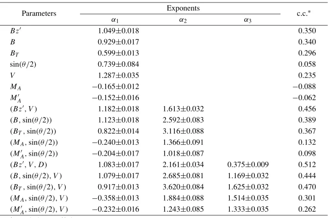
Table 1. Exponents and correlation coefﬁcients (c.c.) for various kinds of solar wind parameters and of their combinations obtained by the regression analysis of the data for the range of−7 ≤ Bz< −1 nT andV < 600 km/s. In this table,(Bz,V,D), for example, represents the case of the regression equation of log(−Q)=const.+α1log(Bz)+α2log(V)+α3log(D). Errors are the standard errors.

Exponents Parameters

α1 α2 α3

c.c.∗

Bz 1.049±0.018 0.350

B 0.929±0.017 0.340

BT 0.599±0.013 0.296

sin(θ/2) 0.739±0.084 0.058

V 1.287±0.035 0.235

MA −0.165±0.012 −0.088

M_A −0.152±0.016 −0.062

(Bz,V) 1.182±0.018 1.613±0.032 0.456

(B,sin(θ/2)) 1.123±0.018 2.592±0.083 0.389

(BT,sin(θ/2)) 0.822±0.014 3.116±0.088 0.367

(MA,sin(θ/2)) −0.240±0.013 1.366±0.091 0.132

(M_A,sin(θ/2)) −0.204±0.017 1.018±0.087 0.098

(Bz,V,D) 1.083±0.017 2.161±0.034 0.375±0.009 0.512

(B,sin(θ/2),V) 1.079±0.017 2.685±0.081 1.169±0.032 0.444

(BT,sin(θ/2),V) 0.917±0.013 3.620±0.084 1.625±0.032 0.470

(MA,sin(θ/2),V) −0.358±0.013 1.884±0.088 1.514±0.035 0.301

(M_A,sin(θ/2),V) −0.232±0.016 1.243±0.085 1.333±0.035 0.262

∗_{correlation coefﬁcient.}

We approximate Eq. (1) by

Q(t)= {Dst∗(t+1 hour)−Dst∗(t−1 hour)}/2

+Dst∗(t)/7.7. (3)

We calculate this quantity for the hourly intervals in which all of the IMF, the solar wind velocity (V), and the density (D) are available. If values calculated from Eq. (3) are positive, we set Q = 0. This is because the ring current is supposed to develop only for negative values of Q. We also impose the following restriction on the y component of the solar wind electric ﬁeld, E y = −BzV (where Bzis measured in the GSM coordinates), according to Burtonet al.(1975):

Q=0 for E y≤0.50 mV/m. (4)

This condition is considered as a cutoff below which the ring current does not develop. We use all negative values of

Qfor the present analysis.

2.2 Procedure of analysis

Procedure of analysis in the present paper is basically the same as that of Aoki (2005) on the AL index.

Figures 1(a) and 1(b) are examples of scatter plots of Q

versus Bz. Data of Fig. 1(a) and those of Fig. 1(b) are for −7 ≤ Bz < −1 nT and V < 600 km/s, and forBz < 0 nT and all V, respectively. Data of Fig. 1(b) also corre-spond to the whole data of the present analysis. As is seen in these ﬁgures, Qdevelops to large negative values asBz

becomes negative. The regression line of Q on Bz, how-ever, usually does not pass through the origin of the Bz-Q

plane, but tends to cross the Bz-axis in the positive side of it. To take account of this tendency, we used the regres-sion coefﬁcients of the regresregres-sion line, Q = a Bz +b, to obtain the value, Bz0 ≡ −b/a, as the value of the point at which the regression line crosses the abscissa. We use

Bz =Bz0−Bzinstead ofBzbelow. This rescaling from

BztoBzis the same as that for the AL index (Aoki, 2005), and is considered as a way of describing the fact that the solar wind-magnetosphere coupling can occur even for the northward IMF conditions. The restriction on the data se-lection, −7 ≤ Bz < −1 nT and V < 600 km/s, was imposed to guarantee that the IMF is directed southward and thus the ring current injection is likely to occur, and to avoid extreme solar wind situations for statistically mean-ingful analyses.

For reference, Fig. 1(c) shows a scatter plot ofQversus

Bz for the data without the condition of (4) and without setting Q =0 even if the value of Eq. (3) is positive. Red points indicate the data for E y ≤ 0.50 mV/m, and blue ones the data for E y >0.50 mV/m. If we remove the data of E y ≤ 0.50 mV/m and those of Q ≥ 0, the remaining data become the same as those of Fig. 1(b). A red line gives the regression line for the data of E y ≤0.50 mV/m,

Q = 0.038Bz−1.313, with a correlation coefﬁcient of 0.029. This very low correlation coefﬁcient implies that there is almost no correlation betweenQandBzforE y ≤

0.5 mV/m.

We performed the regression analysis in the form of

Y =a0X1α1 for each of the following parameters: Bz,B,

BT, sin(θ/2),V, MA, andMA, whereMA andMA are the

Alfven Mach numbers deﬁned in terms ofBT and ofB,

re-spectively, i.e., MA = D1/2V/BT and MA = D1/2V/B.

This was done by the standard regression analysis using the equation logY = loga0 +α1logX1. We also did the re-gression analysis in the formY =a0Xα11Xα22for the follow-ing two-parameter combinations: (Bz,V),(B,sin(θ/2)),

(BT,sin(θ/2)), (MA,sin(θ/2)), and(MA,sin(θ/2)).

Fur-thermore we did the regression analysis in the form Y = a0X1α1Xα

2

2 Xα

3

(4)

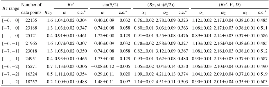
Table 2. Exponents and correlation coefﬁcients (c.c.) forBz, sin(θ/2),(BT,sin(θ/2)), and(Bz,V,D)for various ranges ofBzand forV <600 km/s.

Number of Bz sin(θ/2) (BT,sin(θ/2)) (Bz,V,D)

Bzrange

data points Bz0 α c.c.∗ α c.c.∗ α1 α2 c.c.∗ α1 α2 α3 c.c.∗

[−6, 0] 22135 1.6 1.04±0.02 0.304 0.40±0.09 0.032 0.76±0.02 2.78±0.09 0.323 1.12±0.02 2.17±0.04 0.38±0.01 0.485 [−7, 0] 23188 1.3 1.03±0.02 0.347 0.74±0.08 0.058 0.80±0.01 3.03±0.09 0.363 1.08±0.02 2.17±0.03 0.38±0.01 0.511 [ , 0] 25121 0.4 0.91±0.01 0.461 1.72±0.08 0.129 0.91±0.01 3.55±0.08 0.476 0.89±0.01 2.14±0.03 0.37±0.01 0.586 [−6,−1] 21965 1.6 1.07±0.02 0.307 0.40±0.09 0.032 0.78±0.02 2.88±0.09 0.327 1.13±0.02 2.16±0.04 0.38±0.01 0.485 [−7,−1] 23018 1.3 1.05±0.02 0.350 0.74±0.08 0.058 0.82±0.01 3.12±0.09 0.367 1.08±0.02 2.16±0.03 0.38±0.01 0.512 [ ,−1] 24951 0.4 0.93±0.01 0.465 1.73±0.08 0.129 0.93±0.01 3.62±0.08 0.480 0.90±0.01 2.13±0.03 0.37±0.01 0.587 [−6,−2] 15271 0.7 1.13±0.03 0.306 −0.08±0.12−0.005 1.05±0.02 4.04±0.14 0.330 1.06±0.03 2.10±0.04 0.37±0.01 0.490 [−7,−2] 16324 0.5 1.11±0.02 0.354 0.29±0.11 0.020 1.09±0.02 4.21±0.13 0.374 1.04±0.02 2.09±0.04 0.37±0.01 0.519 [ ,−2] 18257 −0.2 1.00±0.01 0.488 1.48±0.11 0.097 1.14±0.02 4.51±0.11 0.503 0.90±0.01 2.01±0.04 0.35±0.01 0.603

(MA,sin(θ/2),V), and(MA,sin(θ/2),V).

We performed the above analyses under various condi-tions on Bz andV. As the conditions on Bz, we chose the following nine ranges: [−6,0] (which means −6 ≤

Bz < 0 nT; the same format is used throughout this pa-per), [−7,0], [ ,0] (which means Bz < 0 nT), [−6,−1], [−7,−1], [ ,−1], [−6,−2], [−7,−2], and [ ,−2]. As the conditions onV, we examined the following three ranges:

V <600 km/s,V ≥600 km/s, and allV. We analyzed all cases of any combinations of the above BzandV ranges. We will compare the exponents and the correlation coefﬁ-cients in the next section.

3. Results

Table 1 shows the exponents and the correlation coefﬁ-cients for various solar wind parameters and their combi-nations for the range of −7 ≤ Bz < −1 nT and V <

600 km/s. This range of Bz andV is chosen as a typical example. From this table, we notice the following points:

1) The combination (Bz,V,D) shows the highest cor-relation coefﬁcient among the quantities listed in Ta-ble 1.

2) The correlation coefﬁcients for MA, MA, (MA,sin(θ/2)), and (MA,sin(θ/2)) are very low

compared with that forBz, and the correlation coef-ﬁcients for(MA,sin(θ/2),V)and(MA,sin(θ/2),V)

are clearly low compared with that for (Bz,V) and even compared with that forBz.

3) The exponent forBzis about unity in all cases includ-ingBz, i.e., Bz,(Bz,V), and(Bz,V,D).

4) The exponent for sin(θ/2)varies over a wide range for the change in the combination of parameters.

5) The exponent for V varies from about unity to two.

The above features were conﬁrmed to be true for other ranges ofBzandV.

Table 2 shows the examples of the analysis for various kinds of solar wind parameters and their combinations: the exponents and the correlation coefﬁcients for various ranges ofBzand forV <600 km/s. From this table, we notice the following facts:

1) The exponent for Bz is about unity. This character remains valid for the change in the range ofBz. 2) The exponent for sin(θ/2)shows large variability for

the change in the range ofBz.

3) Concerning the combination (Bz,V,D), the expo-nents for Bz, V, and D show almost no variability for the change in the range of Bz; the exponents for

Bz are about unity, those for V are about two, and those for D are about 0.38. It is worth pointing out that these values are very close to the values obtained by Maezawa and Murayama (1986), who showed that the best exponents for Bs(the southward component of the IMF),V, andDare 1.09, 2.06, and 0.38, respec-tively, through the analysis of selected storm events.

We would like to point out one fact. From the present anal-ysis described in the preceding section, we never obtained

B2

Tsin4(θ/2)orB2sin4(θ/2), which is the IMF dependence

expected from theεparameter. This result is the same as that obtained by Aoki (2005) on the AL index. Thus we can conclude that the IMF dependence of theεparameter is never established empirically by the analyses of AL or of

Q.

4. Discussion

4.1 On the validity of the εεεεεεεεparameter and of the Va-syliunaset al.general formula

In this subsection we discuss the validity of theε param-eter and of the Vasyliunaset al.(1982) general formula on the basis of the results of the preceding section.

First, we consider the ε parameter. As mentioned in the last part of the preceding section, we never obtained

B2sin4(θ/2) or BT2sin4(θ/2)by the logarithmic analysis

with restrictions on the values ofBz. Here, we check this result by the linear analysis with restrictions on the values ofθ, not on the values ofBz. We imposed restrictions onθ by 90−10p ≤θ <90+10p◦(p =1,2,· · ·,9), and for each range ofθwe performed the linear regression analysis of QonVl_Bm_sinn_(θ/

2)(l =0,1;m=0,2;n =1,2,4), onVl_B

(5)

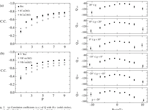
0.0

Fig. 2. (a) Correlation coefﬁcients (c.c.) of Q withBzc(solid circles), with B2_sin4_(θ/₂₎_{(crosses), and with}_B2

Tsin4(θ/2)(open circles) for the ranges of 90−10p≤θ ≤90+10p◦, (p=1, 2,· · ·, 9) and for the range ofV <600 km/s. Values of the abscissa are the values ofp. (b) Correlation coefﬁcients (c.c.) ofQwithV2_Bzc_{(solid circles), with} V B2_sin4_(θ/₂₎_{(crosses), and with}_{V B}2 did this analysis for the following three ranges ofV: V <

600 km/s,V ≥600 km/s, and allV. Figures 2(a) and 2(b)

and BzcV2_{, respectively, for the range of} _V _< ₆₀₀ km/s. From these ﬁgures, general superiority of Bz over

B2_sin4_(θ/₂₎ _{and over} _B2

Tsin4(θ/2)is evident. Other

re-sults (not shown) also support the conclusion thatBzis bet-ter than the combination ofB(orBT) and sin(θ/2).

Next, we consider the general formula of Vasyliu-nas et al. (1982). This formula is derived on the as-sumption that the IMF dependence of the coupling func-tion arises from the Alfven Mach number and sin(θ/2). However, as was pointed out in the preceding section,

MA, MA,(MA,sin(θ/2)), and(MA,sin(θ/2))have much

smaller correlation coefﬁcients with Q than Bz, and

(MA,sin(θ/2),V)and(M_A,sin(θ/2),V)also have clearly smaller correlation coefﬁcients than(Bz,V). These facts

-10

0

10

imply that the Alfven Mach number does not play any im-portant role in the ring current injection and hence in the en-ergy coupling between the solar wind and the Earth’s mag-netosphere. (See Appendix for more detailed discussion.)

Lastly, we discuss the idea that the IMF dependence of the coupling function can be described by the combination of sin(θ/2)and B (or BT). Aoki (2005) pointed out that

this idea has a difﬁculty in expressing the combined effect of the IMF By component and the dipole tilt angle (χ) on the AL index. The reason is as follows: AL develops more efﬁciently for positive Bythan for negative Bywhenχ is negative, and vice versa when χ is positive (Aoki, 1977; Murayamaet al., 1980). Below we refer to this effect as the By-χ effect. This effect is obviously asymmetric with respect to the sign ofBy. Each of the quantities of B,BT,

and sin(θ/2), however, is symmetric with respect to it, so it is impossible to describe theBy-χeffect by the combination

of sin(θ/2)andB(or BT).

Here, we would like to check whether or not Qhas the

(6)

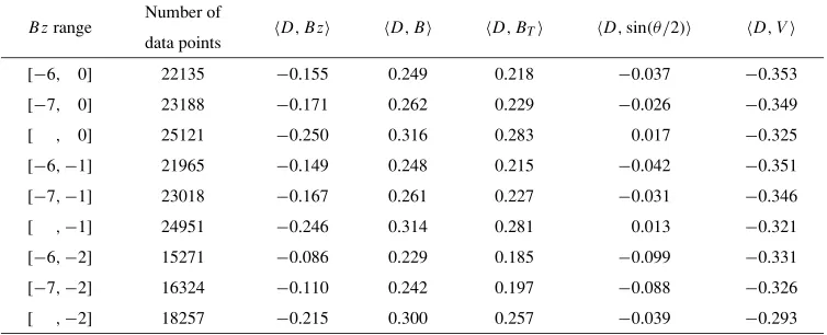
Table 3. Linear correlation coefﬁcients (c.c.) between solar wind parameters for various ranges ofBzand forV <600 km/s. In this table,D,V , for example, represents the case for the linear regression analysis betweenDandV. The same data as those in Table 2 are used for each range ofBz.

Number of

Bzrange

data points D,Bz D,B D,BT D,sin(θ/2) D,V

[−6, 0] 22135 −0.155 0.249 0.218 −0.037 −0.353

[−7, 0] 23188 −0.171 0.262 0.229 −0.026 −0.349

[ , 0] 25121 −0.250 0.316 0.283 0.017 −0.325

[−6,−1] 21965 −0.149 0.248 0.215 −0.042 −0.351

[−7,−1] 23018 −0.167 0.261 0.227 −0.031 −0.346

[ ,−1] 24951 −0.246 0.314 0.281 0.013 −0.321

[−6,−2] 15271 −0.086 0.229 0.185 −0.099 −0.331

[−7,−2] 16324 −0.110 0.242 0.197 −0.088 −0.326

[ ,−2] 18257 −0.215 0.300 0.257 −0.039 −0.293

absolute values ofByincrease in every range ofχ, and that it also tends to develop more efﬁciently for positiveBythan for negativeBywhenχis negative, and vice versa whenχ is positive. ThusQhas theBy-χeffect.

The cause of the By-χ effect is an open question. One possibility is as follows: As pointed out by Murayamaet al. (1980) and by Nakai (1987), we may expect that the location of reconnection at the dayside magnetopause shifts to the pre-noon or post-noon side depending on the sign of the By component of the IMF, and also moves to the summer hemisphere side in association with the variation of χ. According to the By-χ effects of AL and of Q, the period in which AL and Qdevelop more efﬁciently is the time when reconnection occurs on the dawn side of the magnetopause. So we can understand the By-χ effects of AL and of Q by assuming that reconnection on the dawn side of the magnetopause works more efﬁciently than that on the dusk side for some reason.

From the above considerations, we conclude that the ε parameter and the Vasyliunaset al.(1982) general formula are less appropriate than a function of Bz, and that the energy coupling function between the solar wind and the Earth’s magnetosphere is described better by Bz than by the combination of B (or BT) and sin(θ/2). It is worth

mentioning that the above results and conclusions are the same as those obtained by Aoki (2005) through the analysis of the AL index. On the basis of the above results, with attention to the fact that the effect ofByis small compared with that of Bz (cf. Figs. 1 and 3), we suggest that the coupling function,P, is approximated by

P = f(By, χ)BzαVβDγ,

whereα∼1,β ∼2,γ ∼0.4, and f(By, χ)is a function for expressing the effects ofByand ofχ.

4.2 Inﬂuence of the intercorrelations among solar wind parameters

In this subsection we discuss the inﬂuence of the inter-correlations among solar wind parameters on the results.

The intercorrelations amongBz,B,BT, sin(θ/2), andV

were examined by Aoki (2005), and they are not very dif-ferent from the intercorrelations for the data of the present

analysis (not shown). Aoki (2005) did not discuss inter-correlations including the solar wind density because the dependence of the AL index on the density is weak. The solar wind density, however, has a stronger inﬂuence on

Q (cf. Table 1) than on AL, so we examine its intercor-relations here. Table 3 shows the linear correlation coefﬁ-cients for the combinations of(D,Bz), (D,B), (D,BT), (D,sin(θ/2)), and (D,V)for different ranges of Bz and for V < 600 km/s. As is seen in this table, the solar wind density has weak correlations with Bz, B, BT, and V. Among them the intercorrelation between D andV is relatively high (about an anticorrelation betweenV andD, see, e.g., Neugebaur and Snyder, 1966).

The inﬂuence of the intercorrelation between Dand V

and of the strong D dependence of Q can be seen in a rather large difference in the exponent for V between

(Bz,V) and (Bz,V,D). The exponent for V for the case of(Bz,V,D), 2.16, is larger than that for the case of(Bz,V), 1.61 (cf. Table 1); the difference is 0.55. Thus to get the accurate exponent for V we should include the inﬂuence of the solar wind density. This value of about two of the exponent for V supports the quadratic dependence onV (Murayama and Hakamada, 1975; Maezawa and Mu-rayama, 1986), but does not support the linear dependence onV, which is expected from theεparameter.

4.3 Inﬂuence of the assumptions for calculating the ring current injection rate

We have analyzedQderived with some assumptions de-scribed in Section 2.1. In this subsection we discuss the inﬂuence of some of those assumptions on the results.

First, we consider the inﬂuence of the condition on E y, Eq. (4). In order to evaluate this inﬂuence, we calculated a new injection rate without this condition, and performed the same analysis as that in the above. Elimination of the condition of Eq. (4) yielded increase in the number of data points in the small negative Bz ranges, but almost no change in the number of data points in the large negative

(7)

Second, a number of researchers suggested that the decay time is not a constant but has dependence on a parameter: its dependence on the value of Dst (Feldsteinet al., 1984; Gonzalezet al., 1989), and on E y(Fenrich and Luhmann, 1998; O’Brien and McPherron, 2000). We discuss these possibilities here. We investigated the following three decay times suggested by Gonzalezet al.(1989), by Fenrich and Luhmann (1998), and by O’Brien and McPherron (2000):

τG=4 hs for −50 nT≤Dst

We have performed the same analysis as that in the above, and conﬁrmed the validity of all of the features listed in Section 3 and the existence of the By-χ effect for each of the injection rates derived by usingτG,τF L, andτO M,

except for the fact that the exponent forV for the injection rate of τG varies between two and four, being larger than those for the injection rates of otherτ’s.

Here, we would like to point out two facts concerningτG: (1) the value ofτG is rather small compared with those of otherτ’s, and (2) the injection rate ofτGhas a clearly lower linear correlation coefﬁcient withBzthan those of otherτ’s and than that ofτ =7.7 hs. Detailed comparison is beyond the scope of the present paper, and should be discussed in a separate paper.

4.4 On the method of analysis of the present study 4.4.1 On the method of the regression analysis in a logarithmic form In the present study we have examined the dependence of Qon the solar wind parameters, mainly on the IMF, by using the regression analysis in a logarithmic form. In this subsection we discuss the characters of this method and compare them with those of previous studies.

Regression analysis in a logarithmic form has a feature that it can generally deal with every exponent (which is equal to the regression coefﬁcient in this analysis) of pa-rameters of interest, and that it can give the most probable value of each exponent. Coupling functions proposed so far are usually expressed as the products of powers of some so-lar wind parameters, and there are some controversies about values of exponents (e.g.,V versusV2_{). Our method easily} judges the appropriateness of those values of exponents.

Wu and Lundsted (1997a, b) investigated the inﬂuence of the solar wind parameters on the Dstindex by using the neural network method. They showed that the two basic combinations giving accurate prediction are(Bz,V,D)and

(Bs,V,D), and that ε is less appropriate. These results are consistent with ours. In the neural network method, however, an exponent of each parameter should be given before performing the analysis, and so it is not very easy to say what is the most appropriate value of the exponent for the solar wind parameter of interest.

We have investigated the IMF dependence of Qwithout considering detailed dependence ofQonV and onD. This treatment is guaranteed by the fact that the IMF-related pa-rameters (i.e., Bz, B, BT, and sin(θ/2)) have almost no

correlations with V (Aoki, 2005). This treatment is dif-ferent from that of studies in which an exact form of the coupling function including all of the parameters which are assumed to have influence is given first and the validity of this function is examined. Examples of those studies are O’Brien and McPherron (2000) and Temerin and Li (2002). Their purpose is to find out a suitable function that describes the whole time evolution (i.e., the development and the de-cay) ofDst, but our objective is to seek suitable parameters for describing the IMF dependence of the coupling function when the injection occurs, i.e., whenQ<0.

Lastly, we discuss the requirement that the coupling func-tion have the dimension of power (Perreault and Akasofu, 1978; Vasyliunas et al., 1982). It is not necessarily clear that the result of the regression analysis in a logarithmic form meets this requirement. Here, it is worth noting the following two points: First, Q physically reflects the to-tal kinetic energy of the ring current particles through the Dessler-Parker-Sckopke relation (Dessler and Parker, 1959; Sckopke, 1966). However, Q does not have the dimen-sion of power because of its definition of Eq. (1). Sec-ond, what the dimension ofQis is a separate problem from what are parameters controllingQ. If the intensification of the ring current is a result of the solar wind-magnetosphere coupling, Q should show dependence on the same param-eters as those controlling the coupling. Vasyliunas et al.

(1982) assumed that the coupling depends on the Alfven Mach number and on the clock angle. If this assumption is correct,Qshould also depend on those parameters irrespec-tive of the dimension ofQ. (A similar argument can also be applied to the AL index.) The present study addresses the problem of the validity of this assumption, and the regres-sion analysis can give a clear answer to this problem.

4.4.2 Time resolution of the data In the present study we have used hourly values of Q, and often com-pared the results of Q with those of hourly values of AL (Aoki, 2005). In this subsection we discuss the inﬂuence of the time resolution of the data on the result and the physical meaning of the comparison between the results of Q and those of AL.

Studies of the coupling function by using the AE, AL, andDstindices have a long history. Typical analyses of AE or of AL were performed by using 1-min values (e.g., Baker

(8)

been performed before, so it should be done in a future study to check the above idea.

4.5 Previous studies on the Vasyliunaset al. formula and theεparameter

In this subsection we discuss some of previous investiga-tions that dealt with the Vasyliunaset al. general formula andε.

Murayama (1986) analytically derived an equation forQ

in the form ofBsαVβDγ, and compared its exponents with those expected from the Vasyliunas et al.formula. From this comparison he concluded that the values of exponents of his equation are inconsistent with those of the formula. He further suggested that this inconsistency is avoided by introducing an additional multiplicative factor depending onBsV. This procedure, however, is inappropriate because of the following reason: If the Vasyliunaset al.formula is truly a general formula, it should reproduce any dependence observed in the coupling mechanism as a special case with-out introducing an additional factor.

Bargatzeet al.(1986) analyzed the solar wind parameter dependence of the AL index, and showed that AL is ex-pressed byD1/6_V4/3_B_sin4_(θ/₂₎_{, whose exponents are} con-sistent with the Vasyliunaset al. formula. TheirV4/3 de-pendence, however, is weaker than the results of Maezawa and Murayama (1986) and of Aoki (2005), who showed that the exponent forV is close to two. Bargatzeet al.further showed in their Fig. 4(b) that the sin4(θ/2)dependence is a good approximation. Close inspection of this ﬁgure, how-ever, indicates that in the large values ofθ(i.e., negativeBz

ranges),U(θ)cosθ, which corresponds to Bz, agrees bet-ter with the data than sin4(θ/2). The sin4(θ/2)dependence agrees better with the data thanU(θ)cosθ in the smallθ ranges, where the physical meaning of AL is unclear (Allen and Kroehl 1975; Kamide and Akasofu, 1983).

Recently, Koskinen and Tanskanen (2002) thoroughly re-viewed the basic ideas onε, and pointed out some unclear physical foundations on them.

5. Conclusions

We have examined the IMF dependence of the ring cur-rent injection rate calculated from the Dst index by com-paring the inﬂuence of Bz with that of the combination of sin(θ/2)and B (or BT). Main results are as follows: (1)

The exponent forBzshows higher consistency than that for sin(θ/2). Higher consistency is seen in (a) smaller variabil-ity in the exponent for Bz for the change in the range of

Bz, and in (b) much larger variability in the exponent for sin(θ/2)for the change in the combination of parameters. (2) We never obtainB2_sin4_(θ/₂₎_or _B2

Tsin4(θ/2), which is

the IMF dependence expected from theεparameter. (3) The ring current injection rate shows a very low correlation with the Alfven Mach number. (4) The ring current injection rate has theBy-χeffect, which is an effect asymmetric with re-spect to the sign ofBy. From the above results we conclude that theεparameter and the Vasyliunaset al.(1982) general formula are less appropriate than a function ofBz, and that the IMF dependence of the energy coupling function is de-scribed better by Bz than by the combination of sin(θ/2) and B(or BT). The above results and conclusions are the

same as those obtained by Aoki (2005) through the analysis

of the AL index. On the basis of the above considerations, we suggest that the coupling function is approximated by

P = f(By, χ)BzαVβDγ,

whereα∼1,β ∼2,γ ∼0.4, and f(By, χ)is a function for expressing the effects ofByand ofχ.

Acknowledgments. Data of the interplanetary magnetic ﬁeld, the solar wind, and the Dst index were provided by Dr. J. H. King through the WDC-A for Rockets and Satellites in GSFC/NASA.

Appendix.

In this appendix, we supplement the discussion in Sec-tion 4.1 on the Vasyliunaset al.general formula and on the idea that the coupling function is described by the combina-tion of(B(T),sin(θ/2),V,D)with more detailed analysis.

Table A1(a) shows correlation coefﬁcients for MA and

for the combination including MA for various ranges of Bz and for V < 600 km/s. When we compare the cor-relation coefﬁcients with those for(Bz,V,D)in Table 2, we see that(MA),(MA,sin(θ/2)), and(MA,sin(θ/2),V)

have much lower correlations than(Bz,V,D). However, the combination (MA,sin(θ/2),V,D) suddenly shows

great improvement in correlation coefﬁcients compared with(MA,sin(θ/2),V), and the correlation coefﬁcients of (MA,sin(θ/2),V,D) are a little higher, by 0.07 at the

maximum value, than those of (Bz,V,D). (The corre-lation coefﬁcients of (MA,sin(θ/2),V,D)are lower than

(Bz,V,D), as seen in Table A1(b).)

Here we consider the reason for the higher correlation of(MA,sin(θ/2),V,D)than(Bz,V,D). It is worth not-ing the follownot-ing three points: First, in the regression analysis, the result of (MA,sin(θ/2),V,D)is equivalent to that of (BT,sin(θ/2),V,D) in the sense that for

ev-ery range of Bz, exponents for (MA,sin(θ/2),V,D)can be derived from exponents for (BT,sin(θ/2),V,D), and

vice versa. This is easily conﬁrmed by Tables A1(a) and A1(b) and simple calculations. Second, the assump-tion that (MA,sin(θ/2),V,D) works in the solar wind-magnetosphere coupling is not equivalent to the idea that

(BT,sin(θ/2),V,D) works. The latter includes the

for-mer, but the reverse is not true. Third, there is no rea-son that we should include D in the regression analy-sis when we want to judge whether or not the combi-nation (MA,sin(θ/2)) works in the coupling. From the above three points, we cannot interpret that the high cor-relation of (MA,sin(θ/2),V,D) represents the effective-ness of (MA,sin(θ/2)) in the coupling, but should

con-sider that (BT,sin(θ/2),V,D) has a little better

correla-tion than(Bz,V,D). The reasons for the higher correla-tion of(BT,sin(θ/2),V,D)are probably considered as

fol-lows: The effect of Byshown in Fig. 3 can be included in

BT and improve the correlation. Larger number of

param-eters in the combination(BT,sin(θ/2),V,D), 4, than that

of(Bz,V,D), 3, might produce higher correlations. In any case, it should be pointed out again that the idea of describ-ing the coupldescrib-ing by(BT,sin(θ/2),V,D)has a difﬁculty in

expressing theBy-χeffect, as mentioned in Section 4.1.

References

(9)

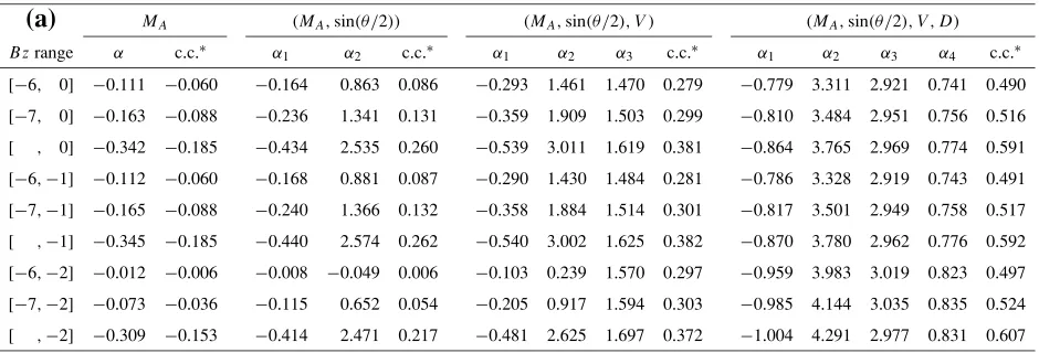
mag-Table A.1. (a) Exponents and correlation coefﬁcients (c.c.) forMA,(MA,sin(θ/2)),(MA,sin(θ/2),V), and(MA,sin(θ/2),V,D)for various ranges ofBzand forV<600 km/s. (b) Same as (a) but for(M_A,sin(θ/2),V,D)and (BT,sin(θ/2),V,D).

(a)

MA (MA,sin(θ/2)) (MA,sin(θ/2),V) (MA,sin(θ/2),V,D)

Bzrange α c.c.∗ α1 α2 c.c.∗ α1 α2 α3 c.c.∗ α1 α2 α3 α4 c.c.∗

[−6, 0] −0.111 −0.060 −0.164 0.863 0.086 −0.293 1.461 1.470 0.279 −0.779 3.311 2.921 0.741 0.490 [−7, 0] −0.163 −0.088 −0.236 1.341 0.131 −0.359 1.909 1.503 0.299 −0.810 3.484 2.951 0.756 0.516 [ , 0] −0.342 −0.185 −0.434 2.535 0.260 −0.539 3.011 1.619 0.381 −0.864 3.765 2.969 0.774 0.591 [−6,−1] −0.112 −0.060 −0.168 0.881 0.087 −0.290 1.430 1.484 0.281 −0.786 3.328 2.919 0.743 0.491 [−7,−1] −0.165 −0.088 −0.240 1.366 0.132 −0.358 1.884 1.514 0.301 −0.817 3.501 2.949 0.758 0.517 [ ,−1] −0.345 −0.185 −0.440 2.574 0.262 −0.540 3.002 1.625 0.382 −0.870 3.780 2.962 0.776 0.592 [−6,−2] −0.012 −0.006 −0.008 −0.049 0.006 −0.103 0.239 1.570 0.297 −0.959 3.983 3.019 0.823 0.497 [−7,−2] −0.073 −0.036 −0.115 0.652 0.054 −0.205 0.917 1.594 0.303 −0.985 4.144 3.035 0.835 0.524 [ ,−2] −0.309 −0.153 −0.414 2.471 0.217 −0.481 2.625 1.697 0.372 −1.004 4.291 2.977 0.831 0.607

(b)

(M_A,sin(θ/2),V,D) (BT,sin(θ/2),V,D)

Bzrange α1 α2 α3 α4 c.c.∗ α1 α2 α3 α4 c.c.∗

[−6, 0] −0.842 2.280 2.536 0.740 0.458 0.779 3.311 2.142 0.351 0.490 [−7, 0] −0.905 2.559 2.583 0.770 0.482 0.810 3.484 2.141 0.351 0.516 [ , 0] −1.043 3.060 2.665 0.830 0.559 0.864 3.765 2.105 0.342 0.591 [−6,−1] −0.844 2.282 2.544 0.740 0.459 0.786 3.328 2.133 0.350 0.491 [−7,−1] −0.907 2.564 2.590 0.771 0.483 0.817 3.501 2.132 0.350 0.517 [ ,−1] −1.046 3.071 2.668 0.831 0.560 0.870 3.780 2.092 0.341 0.592 [−6,−2] −0.820 2.286 2.575 0.722 0.464 0.959 3.983 2.060 0.344 0.497 [−7,−2] −0.905 2.698 2.627 0.762 0.488 0.985 4.144 2.050 0.343 0.524 [ ,−2] −1.079 3.428 2.694 0.836 0.574 1.004 4.291 1.973 0.329 0.607

netic effects of auroral electrojets as derived from AE indices,J. Geo-phys. Res.,80, 3667–3677, 1975.

Aoki, T., Inﬂuence of the dipole tilt angle on the development of auroral electrojets,J. Geomag. Geoelectr.,29, 441–453, 1977.

Aoki, T., On the validity of Akasofu’sεparameter and of the Vasyliunas

et al.general formula for the rate of solar wind-magnetosphere energy input,Earth Planets Space,57, 131–137, 2005.

Baker, D. N., R. D. Zwickl, S. J. Bame, E. W. Hones, Jr., B. T. Tsurutani, E. J. Smith, and S.-I. Akasofu, An ISEE 3 high time resolution study of interplanetary parameter correlations with magnetospheric activity,

J. Geophys. Res.,88, 6230–6242, 1983.

Bargatze, L. F., R. L. McPherron, and D. N. Baker, Solar wind-magnetosphere energy input functions, inSolar Wind-Magnetosphere Coupling, edited by Y. Kamide and J. A. Slavin, pp. 101–109, Terra-pub/Reidel, Tokyo, 1986.

Burton, R. K., R. L. McPherron, and C. T. Russell, An empirical relation-ship between interplanetary conditions andDst,J. Geophys. Res.,80, 4204–4214, 1975.

Dessler, A. J. and E. N. Parker, Hydromagnetic theory of geomagnetic storms,J. Geophys. Res.,64, 2239–2252, 1959.

Fairﬁeld, D. H. and L. J. Cahill, Jr., Transition region magnetic ﬁeld and polar magnetic disturbances,J. Geophys. Res.,71, 155–169, 1966. Feldstein, Y. I., V. Yu. Pisarsky, N. M. Rudneva, and A. Grafe, Ring current

simulation in connection with interplanetary space conditions,Planet. Space Sci.,32, 975–984, 1984.

Fenrich, F. R. and J. G. Luhmann, Geomagnetic response to magnetic clouds of different polarity,Geophys. Res. Lett.,25, 2999–3002, 1998. Gonzalez, W. D., B. T. Tsurutani, A. L. C. Gonzalez, E. J. Smith, F. Tang,

and S.-I. Akasofu, Solar wind-magnetosphere coupling during intense magnetic storms (1978–1979),J. Geophys. Res.,94, 8835–8851, 1989. Gonzalez, W. D., J. A. Joselyn, Y. Kamide, H. W. Kroehl, G. Rostoker, B.

T. Tsurutani, and V. M. Vasyliunas, What is a geomagnetic storm?,J. Geophys. Res.,99, 5771–5792, 1994.

Kamide, Y. and S.-I. Akasofu, Notes on the auroral electrojet indices,Rev. Geophys. Space Phys.,21, 1647–1656, 1983.

Koskinen, H. E. J. and E. I. Tanskanen, Magnetospheric energy budget and the epsilon parameter,J. Geophys. Res.,107(A11), 1415, doi:10.1029/ 2002JA009283, 2002.

Maezawa, K., Statistical study of the dependence of geomagnetic activ-ity on solar wind parameters, inQuantitative Modeling of Magneto-spheric Processes, Geophys. Monogr. Ser., vol. 21, edited by W. P. Ol-son, pp. 436–447, AGU, Washington, D. C., 1979.

Maezawa, K. and T. Murayama, Solar wind velocity effects on the auroral zone magnetic disturbances, inSolar Wind-Magnetosphere Coupling, edited by Y. Kamide and J. A. Slavin, pp. 59–83, Terrapub/Reidel, Tokyo, 1986.

Murayama, T., Coupling function between the solar wind and the Dst

index, inSolar Wind-Magnetosphere Coupling, edited by Y. Kamide and J. A. Slavin, pp. 119–126, Terrapub/Reidel, Tokyo, 1986. Murayama, T and K. Hakamada, Effects of solar wind parameters on the

development of magnetospheric substorms,Planet. Space Sci.,23, 75– 91, 1975.

Murayama, T., T. Aoki, H. Nakai, and K. Hakamada, Empirical formula to relate the auroral electrojet intensity with interplanetary parameters,

Planet. Space Sci.,28, 803–813, 1980.

Nakai, H., Inﬂuence of the transverse component of the interplanetary magnetic ﬁeld on the size of the auroral oval,J. Geomag. Geoelectr.,

39, 501–519, 1987.

Neugebauer, M. and C. W. Synder, Mariner 2 observations of the solar wind, 1, Average properties,J. Geophys. Res.,71, 4469–4484, 1966. O’Brien, T. P. and R. L. McPherron, An empirical phase space analysis

(10)

Geophys. Res.,105, 7707–7719, 2000.

O’Brien, T. P. and R. L. McPherron, Seasonal and diurnal variation of Dst dynamics, J. Geophys. Res., 107(A11), 1341, doi:10.1029/ 2002JA009435, 2002.

Perreault, P. and S.-I. Akasofu, A study of geomagnetic storms,Geophys. J. R. Astron. Soc.,54, 547–573, 1978.

Rostoker, G., H.-L. Lam, and W. D. Hume, Response time of the magne-tosphere to the interplanetary electric ﬁeld,Can. J. Phys.,50, 544–547, 1972.

Sckopke, N., A general relation between the energy of trapped particles and the disturbance ﬁeld near the Earth,J. Geophys. Res.,71, 3125– 3130, 1966.

Temerin, M. and X. Li, A new model for the prediction ofDst on the

basis of the solar wind,J. Geophys. Res.,107(A12), 1472, doi:10.1029/ 2001JA007532, 2002.

Vasyliunas, V. M., J. R. Kan, G. L. Siscoe, and S.-I. Akasofu, Scaling relations governing magnetospheric energy transfer,Planet. Space Sci.,

30, 359–365, 1982.

Wu, J.-G. and H. Lundstedt, Geomagnetic storm predictions from solar wind data with the use of dynamic neural networks,J. Geophys. Res.,

102, 14255–14268, 1997a.

Wu, J.-G. and H. Lundstedt, Neural network modeling of solar wind-magnetosphere interaction,J. Geophys. Res.,102, 14457–14466, 1997b.