L E T T E R
Open Access
The spatial density gradient of galactic cosmic
rays and its solar cycle variation observed with
the Global Muon Detector Network
Masayoshi Kozai
1*, Kazuoki Munakata
1, Chihiro Kato
1, Takao Kuwabara
2, John W Bieber
2, Paul Evenson
2,
Marlos Rockenbach
3, Alisson Dal Lago
4, Nelson J Schuch
3, Munetoshi Tokumaru
5, Marcus L Duldig
6,
John E Humble
6, Ismail Sabbah
7, Hala K Al Jassar
8, Madan M Sharma
8and Jozsef Kóta
9Abstract
We derive the long-term variation of the three-dimensional (3D) anisotropy of approximately 60 GV galactic cosmic rays (GCRs) from the data observed with the Global Muon Detector Network (GMDN) on an hourly basis and compare it with the variation deduced from a conventional analysis of the data recorded by a single muon detector at Nagoya in Japan. The conventional analysis uses a north-south (NS) component responsive to slightly higher rigidity
(approximately 80 GV) GCRs and an ecliptic component responsive to the same rigidity as the GMDN. In contrast, the GMDN provides all components at the same rigidity simultaneously. It is confirmed that the temporal variations of the 3D anisotropy vectors including the NS component derived from two analyses are fairly consistent with each other as far as the yearly mean value is concerned. We particularly compare the NS anisotropies deduced from two analyses statistically by analyzing the distributions of the NS anisotropy on hourly and daily bases. It is found that the hourly mean NS anisotropy observed by Nagoya shows a larger spread than the daily mean due to the local time-dependent contribution from the ecliptic anisotropy. The NS anisotropy derived from the GMDN, on the other hand, shows similar distribution on both the daily and hourly bases, indicating that the NS anisotropy is successfully observed by the GMDN, free from the contribution of the ecliptic anisotropy. By analyzing the NS anisotropy deduced from neutron monitor (NM) data responding to lower rigidity (approximately 17 GV) GCRs, we qualitatively confirm the rigidity dependence of the NS anisotropy in which the GMDN has an intermediate rigidity response between NMs and Nagoya. From the 3D anisotropy vector (corrected for the solar wind convection and the Compton-Getting effect arising from the Earth’s orbital motion around the Sun), we deduce the variation of each modulation parameter, i.e., the radial and latitudinal density gradients and the parallel mean free path for the pitch angle scattering of GCRs in the turbulent interplanetary magnetic field. We show the derived density gradient and mean free path varying with the solar activity and magnetic cycles.
Keywords: Diurnal anisotropy; North-south anisotropy; Heliospheric modulation of galactic cosmic rays; Solar cycle variation of the cosmic ray density gradient
*Correspondence: [email protected]
1Physics Department, Shinshu University, Matsumoto, Nagano 390-8621, Japan
Full list of author information is available at the end of the article
Findings Introduction
A solar disturbance propagating away from the Sun affects the population of galactic cosmic rays (GCRs) in a num-ber of ways. Using Parker’s transport equation (Parker 1965) of GCRs in the heliosphere, we can infer the large-scale spatial gradient of GCR density by measur-ing the anisotropy of the high-energy GCR intensity. This is influenced by magnetic structures such as interplane-tary shocks and magnetic flux ropes in the interplaneinterplane-tary coronal mass ejections (ICMEs). Only a global network of detectors can measure the dynamic variation of the first-order anisotropy accurately and separately from the temporal variation of the GCR density. The Global Muon Detector Network (GMDN) started operation measur-ing the three-dimensional (3D) anisotropy on an hourly basis with two-hemisphere observations using a pair of muon detectors (MDs) at Nagoya (Japan) and Hobart (Australia) in 1992. In 2001, another small detector at São Martinho (Brazil) was added to the network to fill a gap in directional coverage over the Atlantic and Europe. The current GMDN consisting of four multidirectional muon detectors was completed in 2006 by expanding the São Martinho detector and installing a new detec-tor in Kuwait. Since then, the temporal variations of the anisotropy and density gradient in association with the ICME and corotating interaction regions have been ana-lyzed on an hourly basis using the observations with the GMDN (Rockenbach et al. 2014; Okazaki et al. 2008; Kuwabara et al. 2004; Kuwabara et al. 2009).
Solar cycle variations of the interplanetary magnetic field (IMF) and solar wind parameters also alter the global distribution of GCR density in the heliosphere and cause long-term variations of the 3D anisotropy of the GCR intensity at the Earth. The ‘drift model’ of cosmic ray transport in the heliosphere, for instance, predicts a bidi-rectional latitude gradient of the GCR density, pointing in opposite directions on opposite sides of the helio-spheric current sheet (HCS) (Kóta and Jokipii 1982). The predicted spatial distribution of the GCR density has a minimum along the HCS in the ‘positive’ polarity period of the solar polar magnetic field (also referred asA > 0 epoch), when the IMF directs away from (toward) the Sun in the northern (southern) hemisphere, while the distribu-tion has the local maximum on the HCS in the ‘negative’ period (A < 0 epoch) with the opposite field orienta-tion in each hemisphere. The field orientaorienta-tion reverses every 11 years around the period of maximum solar activ-ity. The 3D anisotropy of GCR intensity consists of two components: one lying in the ecliptic plane and the other pointing normal to the ecliptic plane. The ecliptic com-ponent can be observed as the solar diurnal anisotropy (the first harmonic vector of the solar diurnal variation) of GCR intensity, while the normal component can be
measured as the north-south (NS) anisotropy respon-sible for the difference between intensities recorded by north- and south-viewing detectors or the sidereal diurnal anisotropy. By analyzing the solar diurnal variation and the NS anisotropy of the GCR intensity recorded by neu-tron monitors (NMs), Bieber and Chen (1991) and Chen and Bieber (1993) derived the solar cycle variations of 3D anisotropy and modulation parameters on a yearly basis. On the other hand, Munakata et al. (2014) derived the term variation of the 3D anisotropy from the long-term record of the GCR intensity observed with a single multidirectional MD at Nagoya in Japan. By comparing the anisotropy derived from the MD data with that from the NM data, they examined the rigidity dependence of the anisotropy and its solar cycle variation.
1972). The NS anisotropy depends on the polarity of the magnetic field. Based on this fact, Laurenza et al. (2003) showed that the GG-component can be used for deriv-ing reliable sector polarity of the IMF which is defined as
away(toward) when the IMF directs away from (toward) the Sun. By using a global network of four multidirec-tional MDs which is able to observe the NS anisotropy on an hourly basis, Okazaki et al. (2008) reported for the first time that the NS anisotropy deduced from the GG-component is consistent with the anisotropy observed with the global network for a year during the solar activity minimum period.
Analyses of the diurnal variation observed with a sin-gle detector, however, can give a correct anisotropy only when the anisotropy is stationary at least over 1 day and may not work if the anisotropy changes dynami-cally within a day. The GG-component also needs to be averaged over 1 day to cancel the influence of the ecliptic components which have components parallel to the rotation axis of the Earth and contribute to the NS difference measured by the GG-component. Addition-ally, the directional channels of the Nagoya MD have an angular distribution biased toward the northern hemi-sphere, while the GMDN has a global angular distri-bution. It is important, therefore, to examine whether the long-term variation of the 3D anisotropy derived from the conventional analysis of the observed diur-nal variation and the GG-component is consistent with the anisotropy observed by the GMDN which is capa-ble of accurately measuring anisotropy with better time resolution. In this paper, we analyze the 3D anisotropy observed with the GMDN over 22 years between 1992 and 2013 and compare it with the anisotropy observed with the Nagoya multidirectional MD, especially focusing on the NS anisotropy for which the GG-component has been the only reliable measurement at the 50 to 100 GV region. Based on the difference of the response rigidities between the GMDN (approximately 60 GV) and the GG-component (approximately 80 GV), we also discuss the rigidity dependence of the NS anisotropy.
Data analysis
We analyze the pressure-corrected hourly count rateIi,j(t)
of recorded muons in thejth directional channel of theith detector in the GMDN at universal timetand derive three components order anisotropy in the geographic (GEO) coordinate sys-tem by best fitting the following model function toIi,j(t).
Ii,jfit(t)=Ii,j0(t) + ξxGEO(t)
whereI0i,j(t)is a parameter representing the contributions from the omnidirectional intensity and the atmospheric temperature effect;ti is the local time at the ith
detec-tor;c11i,j, s11i,j, andc01i,j are the coupling coefficients; and
ω = π/12. The coupling coefficients are calculated by integrating the response function of atmospheric muons to the primary cosmic rays (Murakami et al. 1979) for primary rigidity, detective solid angle, and detection area with weights of the asymptotic orbit by assuming a rigidity-independent anisotropy with the upper limiting rigidity set at 105GV, far above the maximum rigidity of the response.
In deriving the anisotropy vector ξ, we additionally apply an analysis method developed to remove the influ-ence of atmospheric temperature variations from the derived anisotropy (see Okazaki et al. 2008). Elimination of the temperature effect from the MD data is of particular importance in analyzing the long-term temporal variation ofξ. The deduced anisotropy is averaged over each IMF sector in every month designated as away (toward) if the daily polarity of the Stanford mean magnetic field of the Sun (Wilcox Solar Observatory), shifted 5 days later for a rough correction for the solar wind transit time between the Sun and the Earth, is positive (negative).
We also derive the anisotropy from observations by a single multidirectional MD at Nagoya (hereafter Nagoya MD) which is a component detector of the GMDN. By using the coupling coefficients, we deduce the equato-rial componentξGEO
x ,ξyGEO
ofξfrom the mean diurnal variation of the hourly counting rate in each IMF sec-tor in every month. On the other hand, we derive the normal component to the equatorial plane, ξzGEO, from the GG-component averaged over each IMF sector by using the coupling coefficient in every month (Munakata et al. 2014). The GG-component is a difference combi-nation between intensities recorded in the north- and south-viewing channels and has long been used as a good measure of the NS anisotropy (Mori and Nagashima 1979; Nagashima et al. 1972; Laurenza et al. 2003).
perpendicular (ξ⊥) to the IMF as obtained from the omnitape data and NS anisotropy (ξz) normal to the plane
in each IMF sector in every month. We finally obtain the monthly mean three components of the anisotropy in the solar wind frame as
ξ=ξT
+ξA
/2 (2a)
ξ⊥=ξT ⊥+ξ⊥A
/2 (2b)
ξz=
ξT z −ξzA
/2 (2c)
whereξT
ξA
andξ⊥Tξ⊥Aare parallel and perpendicular components in the ecliptic plane averaged over the toward (away) sector, while ξzT ξzA is the NS anisotropy in the toward (away) sector. We assume that the anisotropy vector, when averaged over 1 month exceeding a solar rotation period, is symmetrical with respect to the HCS which is regarded to coincide with the solar equatorial plane on the average. Because of this assumption, the NS anisotropy is directed oppositely, with the same magni-tude, above and below the HCS as defined in Equation 2c.
Solar cycle variation of the 3D anisotropy
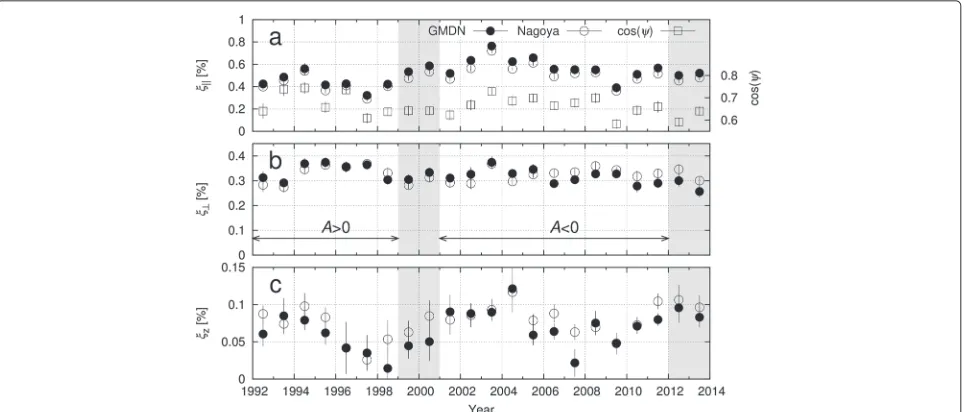
Figure 1a,b,c shows the temporal variations of the yearly mean ξ, ξ⊥, and ξz as defined in Equation 2c,
respec-tively. Each panel shows that the temporal variations of the anisotropy components derived from the GMDN (solid circle) and Nagoya (open circle) data are fairly consis-tent with each other as far as the year-to-year variation is concerned. We can see that the solar cycle variation of
ξhas two components. One is a 22-year variation result-ing in a slightly largerξinA < 0 epoch (2001 to 2011) than inA> 0 epoch (1992 to 1998) as reported by Chen and Bieber (1993). The other is a variation correlated with cosψ, shown withξby open squares in Figure 1a, where
ψ is the IMF spiral angle derived from omnitape data.
ξz deduced from the GMDN (solid circles), on the other
hand, shows an 11-year cycle with minima in 1998 and 2007 around the solar activity minima, whileξ⊥shows no solar cycle variation.
Comparison between the NS anisotropies observed with the GMDN and the GG-component
We now focus on the NS anisotropy which cannot be detected by a single-directional channel separately from GCR density variations. Figure 2 shows histograms of hourly (a and b) and daily (c and d) meanξzGEOobserved by the GG-component (a and c) and GMDN (b and d) in 2006 to 2013, which are classified according to the IMF sectors designated as toward (blue histograms) if
Bx > By and away (red histograms) ifBx < Byby using
the GSE-x, ycomponents (Bx, By) of the IMF vector in
the omnitape data. The blue and red vertical dashed lines represent averages of the blue and red histograms, respec-tively. We define ‘T/Aseparation’ following Okazaki et al. (2008) as
(T−A)/√σTσA
where T (A) andσT (σA) are the average and standard
errors of each histogram in the toward (away) sector,
Figure 1Long-term variations of three components of the anisotropy vector in the solar wind frame.Each panel displays the yearly mean
Figure 2Histograms of the NS anisotropy.Each panel displays the histograms ofξzGEOon(a,b)hourly and(c,d,e)daily bases derived from the
(a,c)Nagoya GG-component,(b,d)GMDN, and(e)NM (Thule-McMurdo) data in 2006 to 2013. Blue and red histograms in each panel represent distributions ofξzGEOin toward and away IMF sectors, respectively, while blue and red vertical dashed lines represent averages of the blue and red histograms, respectively.
respectively. Table 1 listsT−A,√σTσA,T/Aseparation,
and ‘success rate’ (Mori and Nagashima 1979; Laurenza et al. 2003). The success rate is a ratio of the number of hours (days) when the sign of the observedξGEO
z is
posi-tive (negaposi-tive) in the toward (away) IMF sector to the total number of hours (days) and is introduced as a parame-ter indicating to what extent we can infer the IMF sector polarity from the sign of the observedξz. Although we
use the success rate together withT/Aseparation for the following comparison, it is noted that a low success rate does not necessarily imply anything wrong in the observed
ξz. The IMF sector polarity sensed by high-energy GCRs
should be regarded as the polarity averaged over a spatial scale comparable to the Larmor radii of GCRs which span approximately 0.1 AU. It is natural to expect that the IMF polarity averaged over such a large scale does not always
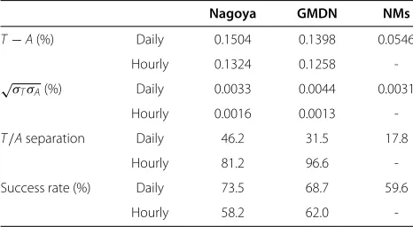
Table 1T−A,√σTσA,T/Aseparation, and success rate
Nagoya GMDN NMs
T−A(%) Daily 0.1504 0.1398 0.0546
Hourly 0.1324 0.1258
-√σ
TσA(%) Daily 0.0033 0.0044 0.0031
Hourly 0.0016 0.0013
-T/Aseparation Daily 46.2 31.5 17.8
Hourly 81.2 96.6
-Success rate (%) Daily 73.5 68.7 59.6
Hourly 58.2 62.0
-Difference (T−A) between averageξGEO
z in toward (T) and away (A) IMF sectors,
geometric mean (√σTσA) of the standard errors ofξzGEOs inTandAsectors, ‘T/A
separation’ (=(T−A)/√σTσA), and ‘success rate’ (see text) derived from Nagoya,
GMDN, and NM (Thule-McMurdo) data in 2006 to 2013 on daily and hourly bases.
follow the single-point measurement of the polarity by a satellite. In Table 1, it is seen that the daily mean ξzGEO by the GMDN shows smaller T/A separation and suc-cess rate than ξGEO
z deduced from the GG-component,
while the hourlyξGEO
z by GMDN has a largerT/A
sep-aration and success rate than the GG-component which has significantly larger dispersion (Figure 2a), partly due to the contribution from diurnal anisotropy as suggested by Okazaki et al. (2008) from their analysis of 1-year data between March 2006 and March 2007.
We also examine the rigidity dependence of the NS anisotropy by analyzing NM data from 2006 to 2013. NMs have median responses to approximately 17 GV GCRs, while the GMDN and GG-component have median responses to approximately 60 GV and approximately 80 GV, respectively. Chen and Bieber (1993) derived the NS anisotropyξzin Equation 2c from the ratio (R) of the
daily mean counting rate recorded by the Thule NM to that recorded by the McMurdo NM as
ξz= b
2
RT −RA
RT +RA (3)
where RT (RA) is the R averaged over toward (away) sectors in every month and b is a constant calculated from coupling coefficients. We define the daily mean NS anisotropy by NMs as
ξGEO
z =
c
2
R
RT +RA (4)
thisξzGEOrepresents those parameters for approximately 17 GV GCRs. The result of this analysis is presented in Figure 2e and Table 1. It is seen that the T/A separa-tion of the NS anisotropy by NMs is significantly smaller mainly due to the smallT −A, i.e., the NS anisotropy is significantly smaller than that obtained from the GMDN and GG-component. The NS anisotropy is smallest in NM data at approximately 17 GV and largest in the GG-component at approximately 80 GV, with the anisotropy in the GMDN at approximately 60 GV in between, sug-gesting that the NS anisotropy increases with increasing rigidity (Munakata et al. 2014).
Solar cycle variation of modulation parameters
Following the analyses by Chen and Bieber (1993), we derive modulation parameters, i.e., the density gradient and the mean free path of the pitch angle scattering. By assuming that the longitudinal gradient is zero in our anal-ysis based on the anisotropy averaged over 1 month which is longer than the solar rotation period, ξ, ξ⊥, and ξz
obtained in Equations 2a, 2b, and 2c are related with the modulation parameters as
ξ = λGrcosψ (5a)
ξ⊥ = λ⊥Grsinψ−RLGz (5b)
ξz = RLGrsinψ+λ⊥Gz (5c)
where RL is the Larmor radius of GCRs in the IMF
and Gz, Gr, λ, and λ⊥ are the latitudinal and radial
density gradients and the mean free paths of the pitch angle scattering parallel and perpendicular to the IMF.
From Equations 5a, 5b, and 5c, we deduce the modulation parameters as
Gz=
αξtanψ−ξ⊥/RL (6a)
Gr=
ξz+
ξ2
z+4αξtanψ
ξ⊥−αξtanψ/(2RLsinψ) (6b)
λ=ξ/ (Grcosψ) (6c)
where α = λ⊥/λ, assumed to be 0.01 and constant as adopted by Chen and Bieber (1993).Gzis converted to the
bidirectional latitudinal gradient as
G|z|= −sgn(A)Gz (7)
whereArepresents the polarity of the solar dipole mag-netic moment and
sgn(A) = +1, forA>0 epoch,
= −1, forA<0 epoch.
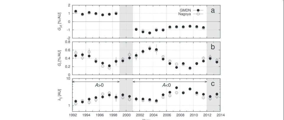
Figure 3a,b,c displays temporal variations of modulation parametersG|z|, Gr, and λ, respectively, obtained from
the GMDN (solid circle) and Nagoya (open circle) data. The variations with 22-year and 11-year solar cycles are clearly seen in this figure. First,G|z| is positive inA > 0
epoch indicating the local minimum of the density on the HCS, while it is negative inA < 0 epoch indicating the maximum in accord with the prediction of the drift model by Kóta and Jokipii (1983). Second, significant 11-year variations are seen in bothGr andλwhich change in a
clear anti-correlation.
Summary and discussions
We analyzed the 3D anisotropy of GCR intensity observed by the GMDN and Nagoya MD in 1992 to 2013. Our analysis of the GMDN data gives the anisotropy on an hourly basis with better time resolution than the traditional analyses of the diurnal and NS anisotropies observed by a single detector such as the Nagoya MD. We confirmed that the 3D anisotropy and the modulation parameters derived from the GMDN and Nagoya MD data are fairly consistent with each other as far as the yearly mean value is concerned. This fact is important particularly for the NS anisotropy derived from the GMDN data, because the GG-component has been the only reliable reference to the NS anisotropy in the rigidity region between 50 and 100 GV.
By analyzing the distribution of the NS anisotropy sep-arately in toward and away IMF sectors, we compared theT/Aseparations and success rates deduced from the GMDN and Nagoya MD data on hourly and daily bases. It is confirmed that the daily mean NS anisotropy observed by the GG-component shows slightly better T/A sepa-ration and success rate than the daily mean anisotropy by the GMDN, while the hourly mean NS anisotropy by the GG-component shows a large spread due to the local time-dependent contribution from the ecliptic anisotropy. The NS anisotropy by the GMDN, on the other hand, shows similar success rate on both daily and hourly bases, indicating that the NS anisotropy is successfully observed by the GMDN, free from the contribution of the ecliptic anisotropy.
In addition to the better time resolution, the new anal-ysis method developed by Okazaki et al. (2008) for the GMDN data also has an advantage of providing the 3D anisotropy, including the NS component, from a single best-fit calculation for intensities recorded by four detec-tors. In contrast, the conventional method using a single MD requires the derivation of the NS anisotropy from the north- and south-viewing channels, separately from the derivation of the diurnal anisotropy using all directional channels.
By comparing the NS anisotropy derived from NM data with those from the GMDN and GG-component data, we find that the NS anisotropy increases with increasing
rigidity and the difference betweenT/Aseparations and success rates of the GMDN and GG-component data is partly due to the rigidity dependence. Yasue (1980) analyzed the GG-component together with the sidereal diurnal variation observed by MDs and NMs and derived the power law-type rigidity spectrum of the average NS anisotropy with a positive power law index of approxi-mately 0.3. By analyzing long-term variations of the 3D anisotropies observed with Nagoya MD and NMs on yearly basis, Munakata et al. (2014) confirmed that the perpendicular component including the NS anisotropy increases with GCR rigidity. If these are the case, the mag-nitude of the NS anisotropy increases with rigidity and theT/Aseparation and success rate will also increase if the dispersion remains similarly independent of rigidity. This is in agreement with our results in Table 1, show-ing that T −Aincreases with the rigidity while√σTσA
is almost constant on a daily basis. Three GCR observa-tions responsible for different rigidities, GG-component (approximately 80 GV), GMDN (approximately 60 GV), and NMs (approximately 17 GV) are capable of observ-ing the NS anisotropy on daily basis, and their cross-calibration allows us to obtain the information about the rigidity dependence of the NS anisotropy.
We confirmed that the solar cycle variations of the yearly mean solar modulation parameters derived from the GMDN and Nagoya data are consistent with each other. The bidirectional latitudinal gradient G|z| shows
a clear 22-year variation being positive (negative) in
A > 0 (A < 0) epochs indicating the local mini-mum (maximini-mum) of the GCR density on the HCS, in accord with the prediction of the drift model (Kóta and Jokipii 1983). On the other hand, significant 11-year solar cycle variations are seen inGr andλ, respectively. The
ecliptic component of the anisotropy ξ parallel to the IMF shows a 22-year variation being slightly larger in
A < 0 epoch (2001 to 2011) than in A > 0 epoch (1992 to 1998) as reported by Chen and Bieber (1993). This variation of ξ is responsible for the well-known 22-year variation of the phase of the diurnal variation (Thambyahpillai and Elliot 1953). We find that the variation of ξ also shows a correlation with the cosψ
Figure 4Long-term variation ofλGrderived from the GMDN data.Yearly mean value and its error are deduced from the average and dispersion of monthly mean values. Gray vertical stripes indicate periods when the polarity reversal of the solar polar magnetic field (referred as
which is governed by the solar wind velocity. This is rea-sonable because ξ is proportional to cosψ as given in Equation 5a. Figure 4 shows yearly variation ofξ/cosψ, i.e.,λGrby the GMDN. In this figure, the 22-year
varia-tion is seen more clearly than in Figure 1 showingξ(Chen and Bieber 1993). For an accurate analysis of the solar cycle variation of the anisotropy, therefore, it is necessary to correct the observed anisotropy for cosψand the solar wind velocity which varies without any clear 11-year or 22-year periodicities.
The 22-year variation ofλGr seems mainly due to the
variation ofλin Figure 3 which is larger inA< 0 epoch (2001 to 2011) than inA>0 epoch (1992 to 1998). How-ever, the solar magnetic field was unusually weak around this last solar minimum (2009), which resulted in a record-high GCR flux (Mewaldt et al. 2010). The larger mean free path is more likely the result of the weaker solar minimum than a polarity issue.
Competing interests
The authors declare that they have no competing interests.
Authors’ contributions
MK, the corresponding author of this paper, made all analyses presented in this paper. KM evaluated the data and discussed the analysis results in this paper. CK made the GMDN data available for this paper. TK made the GMDN data and the neutron monitor data available for this paper. JWB and PE made the neutron monitor data available for this paper. MR kept the São Martinho muon detector in operation. ADL hosted the São Martinho muon detector, assisted with its installation, and performed its general maintenance. NJS contributed in establishing the observation with the São Martinho muon detector and kept it in operation. MT kept the Nagoya muon detector in operation. MLD and JEH hosted the Hobart muon detector, assisted with its installation, performed its general maintenance, discussed the results, and input into the English grammar of this paper. IS established the observation with the Kuwait muon detector. HKAJ and MMS kept the Kuwait muon detector in operation. JK discussed analysis results and worked for improving the English in this paper. All authors read and approved the final manuscript.
Acknowledgements
This work is supported in part by the joint research programs of the Solar-Terrestrial Environment Laboratory (STEL), Nagoya University and the Institute for Cosmic Ray Research (ICRR), University of Tokyo. The observations with the Nagoya multidirectional muon detector are maintained by Nagoya University. CNPq, CAPES, INPE and UFSM support upgrade and maintenance of the São Martinho muon detector. The Bartol Research Institute neutron monitor program, which operates Thule and McMurdo neutron monitors, is supported by National Science Foundation grant ATM-0000315. Wilcox Solar Observatory data used in this study was obtained via the website http://wso.stanford.edu at 2013:06:24$_$22:12:55 PDT courtesy of J.T. Hoeksema. The Wilcox Solar Observatory is currently supported by NASA. JK thanks STEL and Shinshu University for the hospitality during his stay as a visiting professor of STEL.
Author details
1Physics Department, Shinshu University, Matsumoto, Nagano 390-8621, Japan.2Bartol Research Institute, Department of Physics and Astronomy, University of Delaware, Newark, DE 19716, USA.3Southern Regional Space Research Center (CRS/INPE), P.O. Box 5021, 97110-970, Santa Maria RS, Brazil. 4National Institute for Space Research (INPE), 12227-010, São José dos Campos SP, Brazil.5Solar Terrestrial Environment Laboratory, Nagoya University, Nagoya, Aichi 464-8601, Japan.6School of Physical Sciences, University of Tasmania, Hobart, Tasmania 7001, Australia.7Department of Natural Sciences, College of Health Sciences, Public Authority for Applied Education and Training, Kuwait City 72853, Kuwait.8Physics Department, Kuwait University, Kuwait City 13060, Kuwait.9Lunar and Planetary Laboratory, University of Arizona, Tucson, AZ 85721, USA.
Received: 31 March 2014 Accepted: 29 October 2014
References
Bieber JW, Chen J (1991) Cosmic-ray diurnal anisotropy, 1936-1988: implications for drift and modulation theories. Astrophys J 372:301–313 Chen J, Bieber JW (1993) Cosmic-ray anisotropies and gradients in three
dimensions. Astrophys J 405:375–389
King JH, Papitashvili NE (2005) Solar wind spatial scales in and comparisons of hourly wind and ace plasma and magnetic field data. J Geophys Res 110: A02104:1–8
Kóta J, Jokipii JR (1982) Cosmic rays near the heliospheric current sheet. Geopys Res Lett 9:656–659
Kóta J, Jokipii JR (1983) Effects of drift on the transport of cosmic rays. VI. A three-dimensional model including diffusion. Astrophys J 265:573–581 Kuwabara T, Munakata K, Yasue S, Kato C, Akahane S, Koyama M, Bieber JW,
Evenson P, Pyle R, Fujii Z, Tokumaru M, Kojima M, Marubashi K, Duldig ML, Humble JE, Silva MR, Trivedi NB, Gonzalez WD, Schuch NJ (2004) Geometry of an interplanetary CME on October 29, 2003 deduced from cosmic rays. Geophys Res Lett 31: L19803:1–5
Kuwabara T, Bieber JW, Evenson P, Munakata K, Yasue S, Kato C, Fushishita A, Tokumaru M, Duldig ML, Humble JE, Silva MR, Lago AD, Schuch NJ (2009) Determination of interplanetary coronal mass ejection geometry and orientation from ground-based observations of galactic cosmic rays. J Geophys Res 114: A05109:1–10
Laurenza M, Storini M, Moreno G, Fujii Z (2003) Interplanetary magnetic field polarities inferred from the north-south cosmic ray anisotropy. J Geophys Res 108:1069–1075
Mewaldt RA, Davis AJ, Lave KA, Leske RA, Stone EC, Wiedenbeck ME, Binns WR, Christian ER, Cummings AC, de Nolfo GA, Israel MH, Labrador AW, von Rosenvinge TT (2010) Record-setting cosmic-ray intensities in 2009 and 2010. Astrophys J Lett 723:1–6
Mori S, Nagashima K (1979) Inference of sector polarity of the interplanetary magnetic field from the cosmic ray north-south asymmetry. Planet Space Sci 27:39–46
Murakami K, Nagashima K, Sagisaka S, Mishima Y, Inoue A (1979) Response functions for cosmic-ray muons at various depths underground. IL Nuovo Cimento 2C:635–651
Munakata K, Kozai M, Kato C (2014) Long term variation of the solar diurnal anisotropy of galactic cosmic rays observed with the Nagoya multi-directional muon detector. Astrophys J 791: 22:1–16
Nagashima K, Fujimoto K, Fujii Z, Ueno H, Kondo I (1972) Three-dimensional cosmic ray anisotropy in interplanetary space. Rep Ionos Space Res Jpn 26:31–68
NASA (2014) The “omnitape” data accessed on February 10, 2014. http://omniweb.gsfc.nasa.gov/
Okazaki Y, Fushishita A, Narumi T, Kato C, Yasue S, Kuwabara T, Bieber JW, Evenson P, Silva MRD, Lago AD, Schuch NJ, Fujii Z, Duldig ML, Humble JE, Sabbah I, Kóta J, Munakata K (2008) Drift effects and the cosmic ray density gradient in a solar rotation period: first observation with the Global Muon Detector Network (GMDN). Astrophys J 681:693–707
Parker EN (1965) The passage of energetic charged particles through interplanetary space. Planet Space Sci 13:9–49
Rockenbach M, Lago AD, Schuch NJ, Munakata K, Kuwabara T, Oliveira AG, Echer E, Braga CR, Mendonca RRS, Kato C, Kozai M, Tokumaru M, Bieber JW, Evenson P, Duldig ML, Humble JE, Jassar HKA, Sharma MM, Sabbah I (2014) Global muon detector network used for space weather applications. Space Sci Rev 182:1–18
Swinson DB (1969) “Sidereal” cosmic-ray diurnal variations. J Geophys Res 74:5591–5598
Thambyahpillai T, Elliot H (1953) World-wide changes in the phase of the cosmic-ray solar daily variation. Nature 171:918–920
Yasue S (1980) North-south anisotropy and radial density gradient of galactic cosmic rays. J Geomag Geoelectr 32:617–635
doi:10.1186/s40623-014-0151-5