GPS and in situ Swarm observations of the equatorial plasma density irregularities in the topside ionosphere

LETTER

GPS and in situ Swarm observations

of the equatorial plasma density irregularities

in the topside ionosphere

Irina Zakharenkova

_{, Elvira Astafyeva}

_{and Iurii Cherniak}

Abstract

Here we study the global distribution of the plasma density irregularities in the topside ionosphere by using the concurrent GPS and Langmuir probe measurements onboard the Swarm satellites. We analyze 18 months (from August 2014 till January 2016) of data from Swarm A and B satellites that flew at 460 and 510 km altitude, respec-tively. To identify the occurrence of the ionospheric irregularities, we have analyzed behavior of two indices ROTI and RODI based on the change rate of total electron content and electron density, respectively. The obtained results demonstrate a high degree of similarities in the occurrence pattern of the seasonal and longitudinal distribution of the topside ionospheric irregularities derived from both types of the satellite observations. Among the seasons with good data coverage, the maximal occurrence rates for the post-sunset equatorial irregularities reached 35–50 % for the September 2014 and March 2015 equinoxes and only 10–15 % for the June 2015 solstice. For the equinox seasons the intense plasma density irregularities were more frequently observed in the Atlantic sector, for the December solstice in the South American–Atlantic sector. The highest occurrence rates for the post-midnight irregularities were observed in African longitudinal sector during the September 2014 equinox and June 2015 solstice. The observed differences in SWA and SWB results could be explained by the longitude/LT separation between satellites, as SWB crossed the same post-sunset sector increasingly later than the SWA did.

Keywords: Swarm, Plasma irregularities, Topside ionosphere, GPS, Langmuir probe, ROTI

© 2016 The Author(s). This article is distributed under the terms of the Creative Commons Attribution 4.0 International License (http://creativecommons.org/licenses/by/4.0/), which permits unrestricted use, distribution, and reproduction in any medium, provided you give appropriate credit to the original author(s) and the source, provide a link to the Creative Commons license, and indicate if changes were made.

Introduction

After recent reentry of the C/NOFS satellite on Novem-ber 28, 2015, the Swarm becomes the only one satellite mission providing the in situ measurements of the iono-spheric plasma density for altitudes below 550  km. For many decades, in situ plasma probe measurements rep-resent the very important data source for ionosphere research, development and validation of the empirical ionospheric models. Special attention focuses on the plasma density irregularities occurring in the topside ion-osphere (above the ionospheric F2 peak), as only in situ measurements onboard low-earth-orbit (LEO) satel-lites can be used to study the global distribution of these

ionospheric irregularities, their climatology, occurrence probability and other characteristics without taking into account the sparsity of the ground-based facilities and their operational limitation.

Statistical distribution of the plasma density irregu-larities using the in  situ measurements has been stud-ied for many years (e.g., Basu et  al. 1980; Aggson et  al.

1996; Burke et al. 2004; Huang et al. 2014). However, in the conditions of the decrease or lack of the actual in situ data it is important to consider additional information on the properties of the plasma density irregularities, derived from other instruments onboard LEO satellite. Thus, a new method for the ionospheric irregularities detection was successfully implemented using the high-resolution magnetic field measurements onboard the CHAMP satellite (Stolle et  al. 2006; Lühr et  al. 2014). Later, Zakharenkova and Astafyeva (2015) proposed an “additional” use of the precise orbit determination

Open Access

*Correspondence: zakharen@ipgp.fr

(POD) GPS measurements onboard a single LEO satel-lite, CHAMP, for multi-instrumental analysis of the top-side ionospheric irregularities. This GPS POD approach was further successfully developed for multi-satellite use based on an example of quasi-simultaneous Swarm and TerraSAR-X measurements (Zakharenkova et  al. 2015). Therefore, potentially we can obtain additional infor-mation on the global distribution of the plasma density irregularities in the topside ionosphere using GPS meas-urements from LEO missions without LP instrument, like GRACE, MetOP, TerraSAR-X, etc.; however, additional cross-validation analysis on the same database is needed.

The present paper focuses on the comparative analysis of the plasma density irregularities detected in the top-side ionosphere by two independent techniques—GPS and Langmuir probe (LP) measurements. The Swarm mission gives an opportunity to study similarities and dif-ferences between these techniques, as the Swarm satel-lite payload includes both these instruments. The main advantage of the Swarm mission, as compared to previ-ous magnetic mission CHAMP, is that Swarm is a con-stellation of three identical satellites. The latter allows comparison of measurements from identical instruments at different altitudes and in different longitudinal sectors. Also, the GPS and LP data from the Swarm mission have higher temporal resolution than that from CHAMP.

Methods

The GPS POD and LP measurements onboard Swarm Alpha (A) and Swarm Bravo (B) satellites (named hereaf-ter SWA and SWB, respectively) were processed and ana-lyzed in this study. While choosing the time period for our analysis, we take into account that: (1) the commis-sioning phase for the final Swarm orbit configuration was finished on May 2014, (2) from July 15, 2014, the Swarm GPS data are released with 1-s resolution. Therefore, our analysis comprises a period of 18  months from August 2014 to January 2016.

As known, the ionospheric irregularities can be char-acterized by measuring its impact on amplitude and phase of the received GPS signal. Pi et al. (1997) intro-duced into usage for ground-based GPS observations two GPS-based indices: ROT and ROTI. ROT (rate of TEC change) is the time derivative of TEC and is considered as a measure of the phase fluctuation activity. ROTI (rate of TEC index) represents a standard deviation of the ROT over a selected time interval (Pi et al. 1997). The ROTI characterizes the severity of the GPS phase fluctuations and detects the presence of the ionospheric irregularities, and it measures the irregular structure of the TEC spatial gradient. Today, the ROT/ROTI indices, derived from the ground-based GPS data, are widely used in near real-time services of the space weather monitoring (e.g., SWACI

2016) and in investigations of the ionospheric irregulari-ties occurrence at high- and low-latitude regions (e.g., Aarons and Lin 1999; Ma and Maruyama 2006; Jakowski et  al. 2012; Astafyeva et  al. 2014; Cherniak et  al. 2014; Zakharenkova and Astafyeva 2015).

Recently, Zakharenkova et al. (2015) proposed to apply this ROT/ROTI technique to the topside GPS measure-ments from the zenith-looking GPS antenna onboard LEO satellite in order to study the appearance of the plasma density irregularities occurrence in the topside ionosphere (above a LEO orbit altitude). The detailed description of this method implementation for the Swarm GPS data is presented in Zakharenkova et  al. (2015). There are several steps of the GPS data process-ing. First, we calculate a relative slant TEC along all lines of sight Swarm-to-GPS from the frequency-differenced GPS phase delay using the well-known algorithms (Hof-mann-Wellenhof 2001). Initially, the Swarm GPS data were released with 10-s sampling rate, after July 15, 2014, GPS data are provided with 1-s sampling rate. Here we use Swarm GPS data with 1-s resolution. In order to determine the location of the ROT/ROTI results, we used piercing points through a thin layer at the fixed altitude of 500 and 550 km for SWA and SWB, respectively. The ROT is determined by taking the ratio of the difference between the slant TEC values at two successive times to the time interval (Pi et al. 1997). The ROT values are cal-culated and then detrended by subtracting of the running average for all line-of-sight with selected cutoff eleva-tion angle over 30°. The ROT is calculated for each vis-ible GPS satellite over a LEO position in units of TECU/ min, where 1 TECU = 1016 _el/m2_{. The ROTI represents} the standard deviation of the ROT for 15-s interval. In general, the ROT/ROTI technique is a rather simple and straightforward one and it can be promptly transferred to space-borne GPS measurements. However, we should take into account the difference between GPS ROT/ ROTI observed on the ground and aboard a fast-moving platform in space. While ground-based ROT can give a rather clear view on moving ionospheric structures/ irregularities over a fixed GPS station, satellite-based ROT/ROTI might be a mixing of moving structures and rather stationary ionospheric gradients, e.g., equatorial ionization anomaly (EIA).

deviation of the ROD and calculated over 15-s period with sliding window.

Results and discussion

We divide the 18-month data into four seasons related to the June/December solstices and March/September equi-noxes with solstice/equinox month in the middle and one full month before and 1 month after it. We note that data accumulation even for a 3-month period is not enough to cover all 24 h of local time (LT). The average orbit altitude was ~460 and ~510 km for SWA and SWB, respectively.

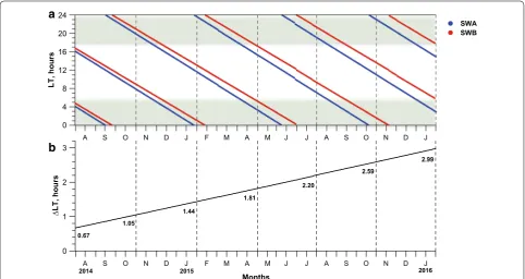
It is important to mention that in the Swarm constel-lation the upper satellite (SWB) slowly separates in local time from the tandem satellites (SWA and SWC). It is a very important issue for this study, as such satellite con-figuration can provide more data for adjacent LT sectors, but can lead to considerable differences in simultaneous comparison of satellites measurements. Figure 1a pre-sents the temporal difference between SWA/SWB satel-lites from August 2014 till January 2016. It is clearly seen how increasing satellites’ separation leads to the differ-ences in LT coverage inside the 3-month intervals. For season of the September 2014 equinox, the LT separation between satellites was about 40–60 min, whereas 1 year later it reached 2.5 h at the equinox of September 2015 and 3 h at the December 2015 solstice (Fig. 1b).

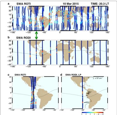
To give the basic idea of the proposed approach, we present overview of ROTI and RODI values calcu-lated from SWA measurements for a case of March 10, 2015 (Fig. 2a, b). Here we used all ascending passes corresponded to the evening sector (~20.3 LT), when in the post-sunset period the equatorial irregularities appear normally. We note that ROTI and RODI values, expressed in the same color-scale, register independently occurrence of the plasma density irregularities in the GPS phase fluctuations above SWA orbit (GPS ROTI, Fig. 2a) and in  situ density variation along SWA orbit (RODI, Fig. 2b). Generally, fluctuations in GPS and LP measure-ments are very small (ROTI below 2  TECU/min) over middle latitudes. More intense fluctuations can be found in the equatorial latitudes, where ROTI/RODI values can reach values of 5–10 and higher. An overview compari-son between concurrent ROTI and RODI results shown in Fig. 2a, b suggests: (1) two independent techniques represent rather similar results; (2) ROTI data distribu-tion, consisted of several satellite-to-satellite passes, has much better spatial coverage comparing to a single pass with in situ measurements. Figure 2c, d shows the ROTI/ RODI values for the SWA pass along 90°W longitude extracted from Fig. 2a, b. In Fig. 2d, we superimpose the variation of the LP-derived in situ Ne values, used for cal-culation of the corresponded RODI variation. This graph

A S O N D J F M A M J J A S O N D J

0 4 8 12 16 20 24

a

b

LT, hou

rs

SWA SWB

A S O N D J F M A M J J A S O N D J

Months

0 1 2 3

LT, hour

s

1.05 0.67

1.44

1.81

2.20

2.59

2.99

5 1 0 2 4

1 0

2 2016

allows us to understand the direct relation between the RODI increases and the appearances of strong depletions in Ne data. At the same time, comparison with ROTI variations (Fig. 2c) shows very similar behavior as in the RODI data, but several ROTI tracks cover much wider area in longitudes than a single RODI track. Therefore, the undoubted advantage of GPS ROTI technique is the fact that while in situ measurements are straightforward

and probe the density point-by-point along a LEO posi-tion, the GPS technique can track simultaneously up to 8–12 different GPS satellites in great spatial volume above a LEO and is able to observe irregularities ahead/ behind/aside LEO position and for much longer time than in  situ cross section. At the same time, the main disadvantage of the GPS ROT/ROTI technique in com-parison with in situ measurements is the integral nature

of GPS TEC measurements making it difficult to local-ize the observed plasma irregularity along the ray path between GPS satellites and a GPS receiver.

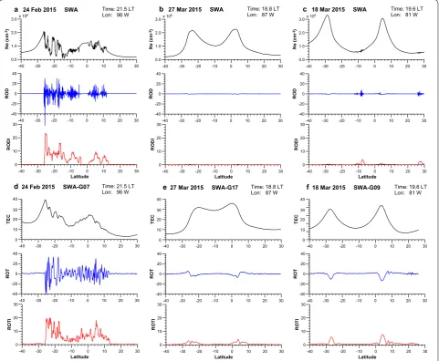
Figure 3 presents several examples of the concurrent LP and GPS data analysis with ROTI/RODI estimation. Figure 3a illustrates the case of the plasma irregularities occurrence in the in  situ Ne measurements (top panel) in the form of the rapid and deep plasma depletions; the detrended ROD variations (middle panel) depict the appearance of the very strong fluctuations at the corre-sponded latitudes with plasma density depletions; index RODI (bottom panel), based on ROD variation, shows a significant increase in absolute values. Figure 3d shows the same case of plasma density detection on February

24, 2015, but in the concurrent GPS measurements. Here we select track between SWA and GPS satellite PRN 07, which due to a favorable GPS orbit configuration was long enough to cover the latitude range of 40°S–30°N. One can see some distortions in the TEC variation (top panel) above 26°S, which are highly correlated with plasma density depletions in Ne data in Fig. 3a. Since topside TEC represents an integral electron content within the whole altitude range of 500–20,200 km, so, it would never contain such steep and deep fluctuations as we can see in one-dimensional horizontal cut of iono-spheric plasma at a fixed altitude when a satellite with LP instrument passes through the plasma density irregulari-ties. So, the integral nature of TEC leads to an attenuated

-40 -30 -20 -10 0 10 20 30

representation of local plasma irregularities or plasma density gradients in the GPS TEC observations com-paring to the in  situ ones. Analysis of the correspond-ing ROT and ROTI values (middle and bottom panels of Fig. 3d) reveals the remarkable agreement with ROD/ RODI values (Fig. 3a) in the form of significant intensi-fication of the GPS TEC fluctuations within the latitude range of 26°S–12°N.

In order to demonstrate the application of the ROTI/ RODI technique during the conditions of the evening-time EIA, non-distorted by the plasma density irregulari-ties, we consider a case of March 27, 2015. Generally, the EIA develops in the low-latitude region as a double band of enhanced ionization at about ±15° magnetic latitude at forenoon hours and then decays gradually until the midnight. In terms of the ionospheric F2 peak height, the EIA is higher in post-sunset than that of the noontime (e.g., Rishbeth 2000; Yue et  al. 2015). This means that during the evening LT the EIA double-peak structure can reach a higher altitude and can be crossed by the Swarm satellites. Obviously, the peak-to-trough difference would be more pronounced in the in situ data than in the top-side TEC above an orbit altitude. Figure 3b, e illustrates a typical example of the well-pronounced EIA during even-ing LT period and quiet geomagnetic conditions, which can be detected by LP and GPS measurements. The cal-culated ROD and RODI values show very weak signa-tures of the double-peak structure, and all RODI values along this latitudinal profile were <1 unit. TEC variation, derived by tracking the GPS PRN 17 satellite, also dem-onstrates the presence of a double-peak structure with less pronounced trough and rather smooth peaks. GPS ROT shows noticeable changes at the TEC peaks loca-tion (middle panel of Fig. 3e), but in form and amplitude they are quite different than in the case of the plasma irregularities occurrence (middle panel of Fig. 3d). ROTI reached maximal values of 2–3 units at the peaks’ lati-tudes, whereas ROTI values outside the peaks are close to zero. Analysis of the data for the evening-time EIA mani-festation in GPS ROTI results  shows that threshold of 3 TECU/min together with a condition of the multi-peak detection is enough to isolate and exclude the impact of the quiet-time EIA on the plasma density irregularities detection in the TEC data.

It should be noted that the EIA could be significantly amplified and uplifted during a severe geomagnetic storm due to the effects of prompt penetration of magneto-spheric electric field and/or disturbance dynamo electric field. To illustrate behavior of the Swarm-derived ROTI/ RODI values during such extreme events, we consider a case of the 2015 St. Patrick’s Day storm, the strongest storm in the current 24th solar cycle. During this storm the significant amplification of the evening-time EIA was

registered in the American and Eastern Pacific regions, from ~22 UT of March 17, 2015, to 03 UT of March 18, 2015, in Ne and GPS TEC data of Swarm satellites (Asta-fyeva et al. 2015). We consider one pass of SWA crossed this sector (longitude of 81°W) at ~01 UT of March 18, 2015. Figure 3c, f presents LP Ne and GPS TEC varia-tions along the SWA pass, respectively. It is clearly seen the EIA intensification with an increase of peak-to-trough difference together with an increase of distance between two peaks. Besides the storm-time EIA develop-ment, it is interesting to note an appearance of the small-scale plasma density irregularities, located outside the peak Ne values close to 8°S and 26°N. These small-scale irregularities are much more pronounced in ROD and RODI variations (middle and bottom panels of Fig. 3c) than rather stationary density gradients corresponded to well-developed EIA crests. The signatures of the EIA crests in the RODI values were <1 unit. As shown in Fig. 3f (top panel), the storm-time enhanced EIA is clearly seen in the topside GPS TEC above SWA altitude and the EIA peaks become very distinct with an increase of the peak-to-trough difference. The signatures of both EIA peaks with a specific shape occur in the ROT and ROTI variations (middle and bottom panels of Fig. 3f). Despite the strong amplification of the evening-time EIA, these quasi-stationary EIA crests appeared in ROTI with maximal amplitude of 4–6 units. Taking into account the obtained results of the extreme ROTI values for the EIA manifestation in quiet and disturbed conditions, for fur-ther analysis we apply a higher threshold of 5 TECU/min together with a condition of the multi-peak detection to exclude impact of the quasi-stationary EIA double-peak structure on the plasma density irregularities detection in the TEC data. Also all days during geomagnetically dis-turbed periods were excluded from the analysis.

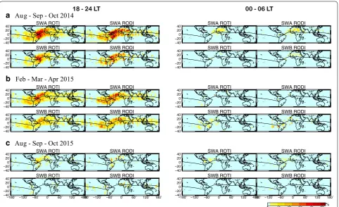
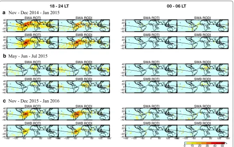
Further, we analyze the seasonal behavior in low- and mid-latitude distribution of the occurrence rate of the density irregularities detected by both GPS-based ROTI and LP-based RODI techniques during August 2014– January 2016. To identify the occurrence of the irregu-larities in the density structure, we set the threshold equal to 2 units for RODI and 5 units for ROTI data. All values, corresponding to the geographical latitude range of 40°S–40°N, were binned and occurrence rate was cal-culated in cells of 2° × 5° resolution in geographical lati-tude and longilati-tude. The temporal range was divided into two periods: the post-sunset and the post-midnight ones which cover 18–24 and 00–06 LT, respectively. Figures 4

separation. There are several features on these figures we need to mention. First, there is a very good agree-ment between the occurrence rate patterns derived from independent GPS and LP techniques. Second, the maximal values of the occurrence rate for the evening-time irregularities were found during equinoxes, in par-ticular for the September 2014 and March 2015 seasons (Fig. 4a, b), and the lowest rates were observed during the June 2015 solstice (Fig. 5b). The maximal occurrence rates were 35–50 % for the September 2014 and March 2015 equinoxes. For the June 2015 solstice, the maximal occurrence rates were 10–15 % and observed in African and Pacific sectors. For the September 2014 and March 2015 equinox, the intense plasma density irregularities were more frequently observed in the Atlantic–African sector (longitudes between 60°W and 60°E), whereas for the December 2014 and December 2015 solstices the zone with the high occurrence rates shifted to the South American–Atlantic sector (longitudes between 120°W and 0°). These results with post-sunset equatorial irregu-larities whose occurrence peak falls on the equinox and lowest values during solstices are in a proper agreement with climatological characteristics of the plasma bubbles

occurrence in the topside ionosphere reported in previ-ous studies (e.g., Burke et al. 2004; Su et al. 2006; Stolle et al. 2006; Park et al. 2013).

One can note that for September 2015 solstice the retrieved values of the occurrence rate were also very low (Fig. 4c, left panel). These differences can be under-stood better if we examine again Fig. 1. The shadow area in Fig. 1 depicts time intervals of 18–06  LT, used here for the occurrence rate estimation. In general, the equa-torial plasma bubbles have been regarded as the typi-cal post-sunset phenomena. They are generated by the growth of the Rayleigh–Taylor instability after sunset (Farley et al. 1970), and their occurrence rate has peak values before midnight. This peak located between 21 and 22  LT during the quiet times for all seasons and during the disturbed times for the March and Septem-ber equinox seasons (Su et al. 2006). The post-midnight equatorial plasma irregularities are relatively rare events; more observations of the post-midnight plasma bub-bles and longitudinally broad depletions (trenches) have been reported recently with the C/NOFS satellite (e.g., Burke et al. 2009; Yizengaw et al. 2013). Thus, the temporal interval of 20–23  LT should provide a major SWA ROTI

contribution to the occurrence rate probability of equa-torial irregularities. As shown in Fig. 1, this temporal interval is properly covered by both satellites only for September 2014 and March 2015 equinoxes, as well as the June 2015 and December 2015 solstices. For the Sep-tember 2015 equinox, the SWA and SWB satellites could not provide enough observations to cover whole post-sunset–midnight period, which can explain rather low values of the occurrence rate. For the December 2014 solstice the SWA and SWB satellites also only partially covered the evening LT sector, but the occurrence rates were rather high and despite the solstice season these estimates were even comparable with those during the March 2015 equinox. During this 3-month period, we have observations for SWA satellite only at 18–20 LT in November 2014 and for SWB—at 18–21 LT in Novem-ber–beginning of December. Other 1.5–2  months did not provide any observations for the evening LT sec-tor at all. However, these available LT intervals coincide well with the time of sunset and peak of the post-sunset irregularities occurrence, which could be the reason for rather high occurrence rates despite the solstice season. Obviously, 1–2  years of the Swarm mission operation is not enough for a climatology study of the occurrence

rate of the equatorial plasma irregularities, as accumu-lated Swarm database does not allow us to get proper LT coverage for each month and, in fact, a 3-month period can depict the occurrence rate referring mostly to a sep-arate month with better coverage of 18–21 LT period.

Comparison of the occurrence rates for the post-sunset and post-midnight periods (left and right panels of Figs. 4, 5) clearly shows  that post-midnight equato-rial irregularities are quite rare phenomena. The high-est occurrence rates for the post-midnight irregularities were observed in the African longitudinal sector dur-ing the September 2014 equinox and June 2015 solstice. Figure 4b (right panel) shows that occurrence rates for the March 2015 equinox were different and much higher at SWB ROTI and RODI values than of SWA ones. As shown in Fig. 1, the SWB values were derived from 00 to 02 LT period during 12 days of February 2015, whereas SWA data for this season consisted of 03–06 LT period in April 2015.

satellite-to-satellite differences. First is an altitude dif-ference of ~50 km between two satellites with possibil-ity that the upper satellite can cross the plasma denspossibil-ity irregularities with lesser intensity than the lower satellite. We should also note that both ROTI and RODI values are based on absolute differences and for the cases of gen-erally lower TEC and Ne values at higher orbit altitudes for SWB satellite the derived ROTI and RODI might be lower here comparing with the lower SWA satellite. The second and more important reason is the temporal/lon-gitudinal separation between the satellites. As shown in Fig. 1, SWA satellite flew in the post-sunset sector earlier than SWB and for the most covered seasons (Septem-ber 2014, March 2015, June 2015 and Decem(Septem-ber 2015) SWA provided more observations for 20–23 LT tempo-ral range. Progressive longitude separation of  the satel-lites becomes more essential for the evening LT sector in February 2015 and reaches more than 1.5 h in LT. This means that SWB satellite appears over the same region up to several hours after SWA and in the case when SWA could be able to cross plasma irregularities near the peak of their occurrence rate, the successive SWB could cross the decaying plasma bubbles and the obtained estimates of the occurrence probability should be lesser for SWB. This difference between SWA and SWB results could be clearly observed while comparing the December 2014 and December 2015 solstices (Fig. 5a, c, right panels), where an increased separation between satellites (from 0.7–1.0 to 2.6–2.9  h) leads to a much smaller values of the occurrence rates derived from the SWB observations.

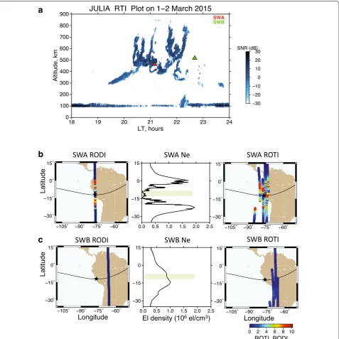
To demonstrate the impact of this temporal/longitudinal separation between the satellites on differences in SWA and SWB observations, we analyze one sample of the post-sun-set equatorial irregularities registered by the JULIA radar at Jicamarca on March 1–2, 2015. Figure 6a shows the JULIA range-time-intensity (RTI) plot with superimposed posi-tion of two Swarm satellites when they passed most closely to the Jicamarca position. One can see that SWA satel-lite (marked by a red triangle) arrived in this region at the time when the post-sunset irregularities were observed at the SWA orbit altitude and rose even up to 700 km. When the SWB satellite arrived in this region with time differ-ence from SWA of about 1.5 h, its pass was more distant from the Jicamarca station as compared to SWA one, but at this LT (near 22.5 LT) the JULIA radar did not registered plasma density irregularities at the whole altitudinal range of 500–900 km. We can expect that both instruments on SWB would reveal quiet level of the irregularities occur-rence. Let’s consider GPS and LP observations for both sat-ellites in more detail. Figure 6b, c shows latitudinal profiles of RODI, electron density Ne and ROTI for SWA and SWB, respectively, when they passed most closely to the Jicama-rca station position. On the SWA RODI profile, we can

recognize two regions of increased values located at both sides from the magnetic equator. Analysis of the SWA Ne profile shows that these high RODI values correspond to the intense plasma density irregularities between the two peaks/crests of the EIA, which was still well defined at that time (21.0–21.5 LT) and at that altitude. At the same time, over the Jicamarca station (marked by asterisk on ROTI/ RODI maps and by green bar on the Ne profile) located within the EIA trough at the magnetic equator, the plasma density fluctuations were generally weak on the SWA Ne profile, as well as on the SWA RODI map. SWA ROTI map shows the appearance of the intense density gradients close to the EIA crests and smaller ROTI values over the Jicama-rca station (marked by black circle). Several passes of GPS satellites close to the magnetic equator had high ROTI val-ues which can be related to the plasma density irregularities seen on the JULIA RTI maps above the SWA orbit altitude (Fig. 6a). Different results were observed for the SWB sat-ellite that came in this sector about 1.5 h later. Most likely due to the reason of LT difference between satellites, or the altitudinal one (~50 km), the SWB Ne profile did not show the crest-trough signatures of the EIA, that had already changed to the normal nighttime behavior characterized by a single peak in the Ne distribution near the geomagnetic equator. No signatures of the intense plasma density deple-tions or gradients can be found in the SWB Ne profile, SWB RODI and SWB ROTI latitudinal profiles at all and, in particular, over the Jicamarca station. These results are con-sistent with the absence of the plasma density irregularities at wide range of altitudes shown on the JULIA RTI plot for Jicamarca. Thus, the progressive temporal separation between the Swarm tandem and the upper satellite will fur-ther reduce the probability that all three satellites could be able to catch signatures of the ionospheric irregularities in the same longitudinal area and/or close to specific ground-based facilities like ionosondes, radars, etc.

Conclusions

Among the seasons with proper data coverage, the maximal occurrence rates for the post-sunset equato-rial irregularities reached 35–50  % for the September 2014 and March 2015 equinoxes and minimal values quite below 10–15 % were found for the June 2015 sol-stice. For the equinox seasons, the intense plasma den-sity irregularities were more frequently observed in the

Atlantic sector, for the December solstice in the South American–Atlantic sector. The highest occurrence rates for the post-midnight irregularities were observed in the African longitudinal sector during the September 2014 equinox and June 2015 solstice. The observed differences in the SWA and SWB results could be explained by the longitude/LT separation between satellites, as SWB

Latitude

Latitude

Longitude _{El density (10}6 _el/cm3_{) Longitude}

SWA SWB

a

b

c

always crossed the same post-sunset sector much later than the SWA did.

The introduced RODI/ROTI technique can be effectively used for an automatic detection of the plasma density irregu-larities caused by the equatorial plasma bubbles occurrence, as well as the plasma density gradients caused by the cross-ing of the quasi-stationary ionospheric structures like peaks of the EIA. One of the undoubted advantages of the LEO ROT/ROTI technique is the fact that while in situ measure-ments are straightforward and probe the density point-by-point along a LEO position, this LEO-based GPS technique can track simultaneously up to 8–12 different GPS satellites in great spatial volume above a LEO and is able to observe irregularities ahead/behind/aside LEO position and for much longer time than in situ cross section. Therefore, even without a LP instrument a LEO satellite with a GPS receiver can offer additional contribution to study the plasma density irregularities occurrence on a global scale.

Authors’ contributions

IZ designed this study, processed and analyzed the GPS data, and wrote the first draft of the paper. EA and IC processed the Swarm LP observations and contributed to the analysis and interpretation of the results. All co-authors contributed to the revision of the draft manuscript and improvement of the discussion. All authors read and approved the final manuscript.

Author details

1 _{UMR CNRS 7154, Institut de Physique du Globe de Paris, Paris Sorbonne} Cité, Univ. Paris Diderot, 35-39 Rue Hélène Brion, 75013 Paris, France. 2 _Space Radio-Diagnostic Research Center, University of Warmia and Mazury, 2 Oczapowskiego, 10-719 Olsztyn, Poland.

Acknowledgements

This work is supported by the European Research Council under the European Union’s Seventh Framework Program/ERC Grant Agreement No. 307998. We acknowledge the European Space Agency (ESA) for providing the SWARM data (http://earth.esa.int/swarm) and the International GNSS Service for GPS orbit products (ftp://cddis.gsfc.nasa.gov). We acknowledge the Jicamarca Radio Observatory for providing the JULIA Radar data through Madrigal Database (jro-db.igp.gob.pe/madrigal/). The Jicamarca Radio Observatory is a facility of the Instituto Geofisico del Peru operated with support from the NSF AGS-1433968 through Cornell University. We thank Stephan Buchert (IRFU) for useful recommendations on the Swarm LP data processing and two anonymous reviewers for their valuable comments and suggestions. This is IPGP contribution 3745.

Competing interests

The authors declare that they have no competing interests.

Received: 31 December 2015 Accepted: 14 June 2016

References

Aarons J, Lin B (1999) Development of high latitude phase fluctuations during the January 10, April 10–11, and May 15, 1997 magnetic storms. J Atmos Solar Terr Phys 61:309–327

Aggson TL, Laakso H, Maynard NC, Pfaff RF (1996) In situ observations of bifurcation of equatorial ionospheric plasma depletions. J Geophys Res 101(A3):5125–5132. doi:10.1029/95JA03837

Astafyeva E, Yasukevich Y, Maksikov A, Zhivetiev I (2014) Geomagnetic storms, super-storms, and their impacts on GPS-based navigation systems. Sp Weather 12:508–525. doi:10.1002/2014SW001072

Astafyeva E, Zakharenkova I, Förster M (2015) Ionospheric response to the 2015 St. Patrick’s Day storm: a global multi-instrumental overview. J Geo-phys Res Sp Phys 120:9023–9037. doi:10.1002/2015JA021629

Basu S, McClure JP, Basu S, Hanson WB, Aarons J (1980) Coordinated study of equatorial scintillation and in situ and radar observations of nighttime F region irregularities. J Geophys Res 75:5119

Burke WJ, Huang CY, Valladares CE, Su S-Y (2004) Longitudinal variability of equatorial plasma bubbles observed by DMSP and ROCSAT-1. J Geophys Res 109(A12):A12301. doi:10.1029/2004JA010583

Burke WJ, de La Beaujardière O, Gentile LC, Hunton DE, Pfaff RF, Roddy PA, Su YJ, Wilson GR (2009) C/NOFS observations of plasma density and electric field irregularities at post-midnight local times. Geophys Res Lett 36:L00C09. doi:10.1029/2009GL038879

Cherniak Iu, Krankowski A, Zakharenkova I (2014) Observation of the iono-spheric irregularities over the Northern Hemisphere: methodology and service. Radio Sci 49:653–662. doi:10.1002/2014RS005433

Farley DT, Balsley BB, Woodman RF, McClure JP (1970) Equatorial spread F: implications for VHF radar observations. J Geophys Res 75:7199–7216 Hofmann-Wellenhof B (2001) Global positioning system: theory and practice.

Springer, New York

Huang C-S, de La Beaujardière O, Roddy PA, Hunton DE, Liu JY, Chen SP (2014) Occurrence probability and amplitude of equatorial ionospheric irregu-larities associated with plasma bubbles during low and moderate solar activities (2008–2012). J Geophys Res Sp Phys 119:1186–1199. doi:10.100 2/2013JA019212

Jakowski N, Béniguel Y, De Franceschi G et al (2012) Monitoring, tracking and forecasting ionospheric perturbations using GNSS techniques. J Sp Weather Sp Clim 2:A22. doi:10.1051/swsc/2012022

Lühr H, Xiong C, Park J, Rauberg J (2014) Systematic study of intermediate-scale structures of equatorial plasma irregularities in the ionosphere based on CHAMP observations. Front Phys 2:1–9. doi:10.3389/ fphy.2014.00015

Ma G, Maruyama T (2006) A super bubble detected by dense GPS network at east Asian longitudes. Geophys Res Lett 33:L21103. doi:10.1029/200 6GL027512

Park J, Noja M, Stolle C, Lühr H (2013) The ionospheric bubble index deduced from magnetic field and plasma observations onboard Swarm. Earth Planets Space 65:1333–1344. doi:10.5047/eps.2013.08.005

Pi X, Mannucci AJ, Lindqwister UJ, Ho CM (1997) Monitoring of global iono-spheric irregularities using the worldwide GPS network. Geophys Res Lett 24(18):2283–2286. doi:10.1029/97GL02273

Rishbeth H (2000) The equatorial F-layer: progress and puzzles. Ann Geophys 18:730–739

Stolle C, Lühr H, Rother M, Balasis G (2006) Magnetic signatures of equatorial spread F as observed by the CHAMP satellite. J Geophys Res 111:A02304. doi:10.1029/2005JA011184

Su S, Liu CH, Ho HH, Chao CK (2006) Distribution characteristics of topside ionospheric density irregularities: equatorial versus midlatitude regions. J Geophys Res 111:A06305. doi:10.1029/2005JA011330

SWACI (2016) The Space Weather Application Center Ionosphere. http://www. swaciweb.dlr.de/data-and-products/?no_cache=1&L=1/. Accessed 15 Mar 2016

Swarm document (2015) Preliminary L1b plasma dataset. http://swarm-wiki. spacecenter.dk/mediawiki-1.21.1/index.php/Preliminary_Level_1b_ plasma_dataset. Accessed 25 Dec 2015

Yizengaw E, Retterer J, Pacheco EE, Roddy P, Groves K, Caton R, Baki P (2013) Postmidnight bubbles and scintillations in the quiet-time June solstice. Geophys Res Lett 40:5592–5597. doi:10.1002/2013GL058307

Yue X, Schreiner WS, Kuo YH, Lei J (2015) Ionosphere equatorial ionization anomaly observed by GPS radio occultations during 2006–2014. J Atmos Solar Terr Phys 129:30–40. doi:10.1016/j.jastp.2015.04.004

Zakharenkova I, Astafyeva E (2015) Topside ionospheric irregularities as seen from multisatellite observations. J Geophys Res Sp Phys 120(1):807–824. doi:10.1002/2014JA020330