R E S E A R C H
Open Access
Multi-antenna spectrum sensing by exploiting
spatio-temporal correlation
Sadiq Ali
1,2*, David Ramírez
3, Magnus Jansson
4, Gonzalo Seco-Granados
1and José A López-Salcedo
1Abstract
In this paper, we propose a novel mechanism for spectrum sensing that leads us to exploit the spatio-temporal correlation present in the received signal at a multi-antenna receiver. For the proposed mechanism, we formulate the spectrum sensing scheme by adopting the generalized likelihood ratio test (GLRT). However, the GLRT degenerates in the case of limited sample support. To circumvent this problem, several extensions are proposed that bring robustness to the GLRT in the case of high dimensionality and small sample size. In order to achieve these sample-efficient detection schemes, we modify the GLRT-based detector by exploiting the covariance structure and factoring the large spatio-temporal covariance matrix into spatial and temporal covariance matrices. The performance of the proposed detectors is evaluated by means of numerical simulations, showing important advantages over existing detectors.
Keywords: Cognitive radio; Generalized likelihood ratio test (GLRT); Multi-antenna; Spatio-temporal correlation
1 Introduction
For a cognitive radio system, which opportunistically accesses the wireless channel, spectrum sensing becomes a crucial task for detecting the presence of primary user transmissions [1]. Recently, sensors with multi-ple antennas have become an integral part of many cognitive receivers [2,3], thus giving us the chance to consider multi-antenna techniques to improve the per-formance of spectrum sensing. Multiple antennas can offer spatial diversity and improve the spectrum sens-ing performance [4,5]. Intuitively, the presence of any primary signal should result in some spatial correla-tion in the observacorrela-tions received at the multi-antenna receivers [5] and thus, exploiting this correlation improves the primary user detection performance. In addition to being spatially correlated, the received signal sam-ples are usually correlated (wide-sense stationary) in time due to presence of a temporal dispersive chan-nel, oversampling of the received signals or just because the originally transmitted signals are correlated in time
*Correspondence: [email protected]
1SPCOMNAV, Universitat Autònoma de Barcelona, 08193 Bellaterra, Barcelona, Spain
2Electrical Engineering, University of Engineering and Technology, Peshawar, 25000 Peshawar, Pakistan
Full list of author information is available at the end of the article
[5,6]. This spatio-temporal correlation is a feature that can be used for detection purposes, since the remaining (i.e. undesired) noise processes at different antennas can be safely assumed statistically independent, both in time and space.
Spectrum sensing methods that only exploit the spa-tial structure of the received signal covariance matrix have been of great interest in the recent years [5]. The majority of these schemes are based on multivariate sta-tistical inference theory [7,8], and interested readers can find comprehensive details in ([8], Ch. 9-10), which dis-cusses multivariate detectors for testing the independence of random observations with the help of the generalized likelihood ratio test (GLRT). These GLRT-based detectors typically end up in a simple quotient between the determi-nant of the sample covariance matrix and the determidetermi-nant of its diagonal version, and these tests have been widely applied to the detection of signals especially in the context of cognitive radios [2,9].
Through careful study of various existing spectrum sensing techniques, one can conclude that the signal’s temporal correlation is not fully exploited in most of these techniques. In fact, in most of them, temporal correlation is ignored or considered as a deleterious effect. In the very few works that exploit the temporal correlation, they usually assume some prior knowledge about it [10-14].
One of the reasons for ignoring or only partially exploit-ing temporal correlation is that it often makes it difficult to achieve tractable solutions. However, the exploitation of temporal correlation jointly with spatial correlation can provide us extra side information to enhance the detec-tion performance. Hence, it will be interesting to find ways to devise detection mechanisms that exploit tempo-ral correlation with tractable solutions. Taking this into account, the main focus of this work is to develop a multi-antenna detector that robustly exploits spatio-temporal correlation. In order to do so, we propose a signal model that leads us to tractable detection schemes while exploiting the temporal correlation jointly with spatial correlation.
In order to achieve the proposed goal, we start with our earlier work in [15], where we derived the GLRT. This detector basically tests whether the covariance matrix is block diagonal or not. To make the discussion and notation simple, for our case, we call this GLRT scheme the spatio-temporal GLRT (ST-GLRT). Compared to the traditional spatial covariance-based GLRT, the ST-GLRT provides some improved performance. The reason for this is that the ST-GLRT scheme exploits temporal correla-tion as an addicorrela-tional feature on top of spatial correlacorrela-tion and energy. However, since any GLRT involves the estima-tion of unknown parameters (e.g., covariance matrix), its performance depends on the sample size and the dimen-sionality of the signal model. In practice, the GLRT is used based on the assumption that the sample size is large compared to the model dimension. When this is not the case, the performance of the GLRT degenerates because the sample covariance matrix becomes singular, and the whole problem becomes ill-conditioned [16,17]. In the case of the ST-GLRT, we have to deal with both the spa-tial and temporal dimensions, and hence, the overall data dimension is even larger. Thus, the ST-GLRT has some further limitations when the detection process requires a quick decision, as it is in the case of the detection of pri-mary signals in cognitive radio. Hence, although for the large sample support, the ST-GLRT can certainly achieve an improved detection performance; for small sample support, it has some limitations that deserve a detailed study.
In order to reduce the demand for large sample sup-port and bring robustness to the ST-GLRT, one may assume existence of some underlying structure based on the spatial and temporal components of the covariance matrix. In our earlier work [15,18], by assuming wide sense stationary (WSS), we exploited the Toeplitz struc-ture of the covariance matrix. Doing so, we proposed an approximated GLRT in the frequency domain that leads to robustness against the small sample support. Contrary to that work, in the present one, we rather focus on exploiting the covariance structures without the GLRT
approximation in the frequency domain. In particular, we approximate the block-Toeplitz structure of a multivari-ate WSS process as persymmetric. Doing so, we will take advantage of the result in [19] which states that by exploit-ing the persymmetric structure, the number of indepen-dent vector measurements required for the covariance matrix estimator can be decreased by up to a factor of two. This will certainly bring down the demand for high sam-ple support required for the ST-GLRT to not degenerate and provide robustness against the repercussions of small sample support and large dimensional data.
Moving one step forward, we also approximate the block-Toeplitz structure of the spatio-temporal correlated multi-antenna measurements with a Kronecker product structure [20,21]. Recently, exploitation of the Kronecker structure in covariance matrices has received a lot of interest in statistics [22,23]. Moreover, the maximum like-lihood (ML) method for estimating the covariance matrix based on the Kronecker product has been previously discussed in [22,23]. Similarly, in the cases where the correlation structure is not separable through the Kro-necker product, [24] discusses some insightful details about the nearest Kronecker product approximations. In this paper, we use the Kronecker structure to reformu-late the ST-GLRT by taking advantage of the inherent spatio-temporal structure of the received observations. In order to do so, we adopt and extend our earlier work [25] by using the Kronecker product to efficiently exploit the space-time correlation in a multi-antenna spectrum sensing scheme. In addition to the Kronecker product-based factorization, we also exploit the fact that the fac-tored matrices could have additional persymmetric struc-ture [21]. Therefore, by exploiting the Kronecker product structure jointly with the persymmetric structure, the per-formance of the proposed detection scheme can further be improved in terms of the required number of sam-ple to estimate the covariance matrix (i.e. the detector efficiency).
To compare the proposed methods with traditional techniques, numerical simulations are conducted. These results illustrate that the proposed detection schemes indeed outperform the traditional approaches, especially in the case of small sample support.
The remainder of the paper is organized as follows. Section 2 introduces the proposed methodology and the signal model. In Section 3, we solve the problem by using the traditional GLRT formulations. The proposed detec-tion schemes are derived in Secdetec-tions 4 and 5. Numerical results are provided in Section 6. The conclusion is finally drawn in Section 7.
2 Proposed methodology and signal model
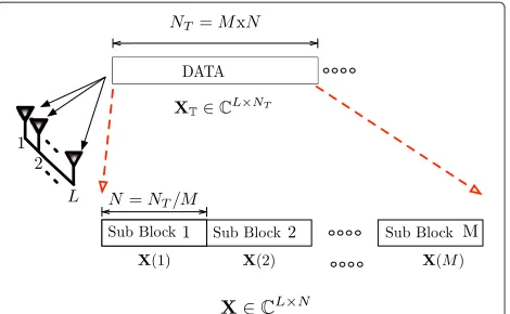
is equipped with L antennas as shown in Figure 1. We assume no prior knowledge about the primary transmis-sion or the noise processes except that the noise is spatio-temporally independent. We focus on a practical scenario where due to the presence of a primary user (PU) signal, the received signals at the Lantennas are correlated in space as well as time. The spatial correlation is due to the proximity between the receiving antennas and the tempo-ral correlation is due to the presence of a tempotempo-ral dis-persive channel, oversampling of the received signal or the time correlation of the transmitted signal [6]. In this work, we consider the temporal correlation to be WSS. Hence, consecutive received samples of the(L×1)vectorx(n), n=1,. . .,NT atLantennas of a user are temporally cor-related, wherex(n)[x1(n),x2(n),. . .,xL(n)]TandNT is the total number of received vector samples. Exploiting the temporal correlation, jointly with spatial correlation, can provide us extra information to enhance the detection performance. In order to devise detection mechanisms that exploit temporal correlation with tractable solutions, the proposed technique can be described as follows:
1. We split the received block ofNTvectorsx(n)into Msub-blocks where each block containsNsamples of vectorx(n), as shown in Figure 2.
2. We assume that the consecutive vector-valued samples within each sub-block are temporally correlated withN×Ntemporal correlation matrixCt.
3. Independence is assumed between consecutive sub-blocks.
It is clear that the proposed approach does not exploit the correlation among different sub-blocks. However, as it will become clear in the following sections, exploit-ing such correlation would result in an ill-posed prob-lem. This would make it intractable to derive the ML estimators of the covariance matrices, required for the generalized likelihood ratio test (GLRT). The proposed
Figure 1System model for a single secondary user equipped with multiple antennas and multi-antenna primary user.
Figure 2Schematic representation of the proposed methodology for slicing the observation block intoMsub-blocks.
mechanism could also be motivated from the concept of correlated block-fading channel, which presents correla-tion in eachN-samples block, but independence between consecutive blocks [6,26].
In order to proceed, we need the distribution of {x(n)}NT
n=1, and we assume it to be zero-mean complex Gaussiana. This assumption is particularly reasonable if the primary network employs orthogonal frequency divi-sion multiplexing (OFDM) as modulation format [15,18]. Similarly, we also assume that the SU collectsNT consec-utive samples of vectorx(n). Based on the proposed three step approach discussed above, the received NT vector samples are divided intoMblocks and each block consists ofNvector samples, such thatMN=NT. Them-th block is defined as:
X(m)
= ⎡ ⎢ ⎢ ⎣
x1(1+(m−1)N) x1(2+(m−1)N) · · · x1(N+(m−1)N)
x2(1+(m−1)N) x2(2+(m−1)N) · · · x2(N+(m−1)N)
... ... ... ...
xL(1+(m−1)N) xL(2+(m−1)N) · · · xL(N+(m−1)N) ⎤ ⎥ ⎥ ⎦
= ⎡ ⎢ ⎢ ⎢ ⎣
xT1 (m) xT2 (m)
...
xTL(m) ⎤ ⎥ ⎥ ⎥ ⎦,
(1)
where thei-th row,xTi (m)form=1,. . .,M, contains N-samples at thei-th antenna. Let us define a vectorz(m) vecXT(m) . The covariance matrix of theLN×1 vector z(m)under hypothesisH1is
=E
zzT
=
⎡ ⎢ ⎢ ⎢ ⎣
11 12 · · · 1L 21 22 · · · 2L
... ... ... ...
L1 L2 · · · LL
⎤ ⎥ ⎥ ⎥
⎦∈CLN×LN,
where the sub-block covariance matricesil=E the hypothesis testing problem becomes
H0:z∼CN(0,0),
H1:z∼CN(0,).
(3)
Now, considering that the noise powers at theL anten-nas of the user are different and spatially and temporally uncorrelated noise, the covariance matrix under noise-only hypothesis is0=A,0⊗IN, where
3 GLRT based on spatio-temporal correlation
In this section, by adopting the GLRT formulation, we review a spectrum sensing scheme that exploits both the spatial and temporal correlation without exploiting any a-priori structure. This will be done just to provide a reference benchmark to compare the proposed detectors in Sections 4.2 and 5. Since, the parameters{0,}are unknown, we need to adopt the GLRT approach and the test statistic of the ST-GLRT can be formulated as:
ST(Z)= under hypothesis H0 and H1, respectively. We assume that we have M independent blocks of the data X, or equivalently vector z, Z z(1) z(2), · · ·, z(M) available. To solve the GLRT (5), we have to derive the ML estimators of the parameters for each of the hypothe-ses. Note that under weak conditions, the ML estimator is asymptotically an unbiased and efficient estimator [27]. The expression for the likelihood function fz(Z;)under hypothesisH1can then be written as:
fz(Z;)= 1
(π)MLN||Mexp
−Mtr−1ˆ. (6)
Taking into account that has no further structure beyond being positive semi-definite, it is easy to prove [7] that its ML estimate is given by the sample covariance
matrix i.e. ˆ = M1 Mm=1z(m)zH(m). Under the
alter-Now, taking into account the Kronecker structure of the covariance matrix, (7) may be rewritten as [25]:
fz(Z,0)=fx and the ML estimate of the covariance matrix A,0 becomesˆA,0= diag expression of the ST-GLRT becomes:
ST(Z)=
Note that the detection scheme in (9) assumes no struc-ture for the covariance matrix, except that the covariance matrix is Hermitian and non-singular.
Solving (10), the final expression of the detector that does not exploit the temporal structure is
Tr(XT)= matrix. Under the hypothesisH0, as we have previously shown, the covariance matrix may be estimated as:A,0= diagA,1 [7]. The detector (11) only exploits the energy and the spatial correlation across theL antennas of the receiver and it wrongly assumes independence in time the information provided by the temporal correlation. Compared to (11), the ST-GLRT (9) provides improved detection performance since it uses temporal correlation as an additional source of information. However, in the case whenM < NL, the ST-GLRT may completely col-lapse due to the ill-conditioned sample covariance matrix [17]. In order to circumvent this limitation, in the fol-lowing sections, we propose some modifications in the ST-GLRT by exploiting the presence of some inherent structures in the space-time correlation.
4 Exploiting persymmetric structure
In order to solve the detection problem (3) with unknown covariance matrices, a critical requirement for the detec-tors based on the GLRT is that the sample covariance matrices must be non-singular [23]. To this end, we have to make sure that the number of available observations given by M, is not smaller than LN (i.e. M ≥ LN). However, in quick spectrum sensing, a number of sam-ples greater thanLNis a requirement difficult to fulfill in practice [28]. Hence, the motivation of the remaining dis-cussion is to bring robustness against this small sample support. Note that in (9) we assume no prior knowl-edge about the spatio-temporal structure of the covari-ance matrix except that it is positive definite. One way to achieve the robustness against the small sample support is to look for possible a-priori known patterns/structures in the large spatio-temporal covariance matrix.
4.1 Persymmetric structure
In this section, we use the fact that the spatio-temporal covariance matrixhas a persymmetric structure. From [15,18], we know that the multivariate WSS time series has a block-Toeplitz covariance matrix. We remark here that Toeplitz structured matrices belong to a subclass of the persymmetric matrices [19,21,29]. Furthermore, considering structured antenna array configurations (i.e., uniform linear arrays) at the SU, the spatio-temporal covariance matrixcan be modelled as persymmetric-block-Toeplitz, as shown in [30]. Therefore, we propose to approximate the spatio-temporal covariance matrix,
which is block-Toeplitz, as a persymmetric matrix. Obvi-ously, this approximation results in a suboptimal detection scheme, but it is well known that it does not exist in closed-form ML estimators for Toeplitz matrices. More-over, it provides better detection performance than the unconstrained ML estimate, particularly, in the case of small sample support. Persymmetric covariance matrices fulfill [31]
=JLNTJLN, (12)
where theLN×LNcounter-identity matrixJLN is
JLN =
also known as exchange matrix [19]. Based on these ideas, in Section 4.2, we present a modified GLRT that exploits the persymmetric property of the block-Toeplitz covari-ance matrix.
4.2 Persymmetric GLRT (P-GLRT)
The difference in the formulation of the GLRT that exploits the persymmetry comes due to the constraint (12). Therefore, the formulation of the GLRT based on the persymmetric covariance matrix can be represented as:
PS(Z)=
Comparing (14) to (5), we can see that the differ-ence lies only in the denominator. In order to exploit the persymmetry of , we need to use the forward-backward (FB) log likelihood [32], which is a combination of the forward-looking and the backward-looking log-likelihood functions. The forward-looking log-log-likelihood logfz(Z;)can be written as:
logfz(Z;)= −log|| −tr
−1ˆ, (15)
where we have ignored constant terms that do not depend on data. Similarly, using the constraint = JLNTJLN,
where
The covariance matrix estimator (18) is called forward-backward sample covariance matrix, which is the ML estimator of the persymmetric covariance matrix [32]. An exact theory indicating the performance of the estima-tor as a function of number of independent vecestima-torz(m), m = 1, 2,. . .,M, is not available. However, a qualitative discussion reported in [19,29] shows that the required number of samples decreases by approximately a factor of two. Similarly, it is reported in [33] thatˆPShas con-sistently lower variance than the variance of ˆ. Finally, solving (14) and using (18), the GLRT becomes
PS(Z)= tion scheme in (9), the new one in (19) offers improved performance at small sample support, as the number of independent vector measurements required for the covariance matrix estimator decreases by up to a factor of two [19]. Motivated by these facts, in Section 5, we go one step further and exploit the properties of the Kro-necker product to decompose the large covariance matrix into smaller ones, reducing considerably the number of unknown parameters.
5 GLRT based on Kronecker factorization
In Section 3, we presented the ST-GLRT approach for the detection problem in (3) and argued that it performs poorly forM < KN. In Section 4.1, we have (partially) exploited the temporal structure by imposing persym-metry on the covariance matrix. We have also discussed that the spatio-temporal covariance matrixhas block-Toeplitz (with block-Toeplitz blocks) structure. In [34,35], it is reported that the block-Toeplitz structure can be approx-imated by the Kronecker product of two matrices. Taking this into account, we therefore approximate the covari-ance matrixinto a purely spatial and a purely temporal component as:
=A⊗T. (20)
In (20), the matrixAcaptures the spatial correlation between the observations received at different antennas and matrixT captures the time correlation betweenN column vectors inX. Herein, we remark that the covari-ance structure in (20) makes the implicit assumption that the temporal correlation structure remains the same at all
spatial locations. Similarly, the spatial correlation struc-ture remains the same for the whole sub-block.
5.1 KR-GLRT
In this section, we consider the Kronecker product-based factorization and derive the GLRT that exploits this struc-ture, which is given by
KR(Z)=
estimate of T fixed and vice versa. In [23], numerical experiments show that the Flip-Flop algorithm performs very well and is much faster than a more general pur-pose optimization algorithm such as Newton–Raphson [23]. In [22], it has been reported that for the case of large enoughM, asymptotic efficiency of the ML approach can be achieved without iterating. Moreover, it is reported in [23,36] that if(M−1)N ≥ Land (M−1)L ≥ N, or equivalently M ≥ max(N/L;L/N) + 1, then every iterate in the Flip-Flop algorithm results in positive defi-niteˆA⊗ˆT with probability one. Taking into account this fact, in order to get , we adopt a non-iterativeˆ Flip-Flop approach and only perform the steps given in Algorithm 1, with an initial value ofˆ0A = IL×L. On the other hand, underH0, we have the estimate of0as:ˆ0=
ˆ
A,0⊗IN×N. Having all of the maximum likelihood-based estimates, and solving (21), we can get the expression:
Algorithm 1 ML based Non-Iterative Flip-Flop
• Choose a starting value for ˆ0A as IL×L.
• Estimate ˆ1T from (25) with ˆA=ˆ0A.
• Find the following
1. Estimate ˆA from (26) with ˆ1T.
The main advantage of the proposed GLRT (27) over the traditional is that underH1instead of 12LN(LN+1) parameters, it has only12L(L+1)+ 12N(N+1) parame-ters to estimate. Furthermore, the dimensions of these two covariance matrices T andA are much smaller than the dimension of full covariance matrix , that is why the computations are much less demanding. Hence, the Kronecker model is a good approximation that captures important information about the correlations, while it is positive definite forM≥max(N/L;L/N)+1, i.e. a much smaller number of samples.
5.2 PK-GLRT
In Section 4, we have assumed that the covariance matrix has a block-Toeplitz (with Toeplitz blocks) structure. Keeping this in mind, in this section, we assess the possible improvement in the detection performance of
(27) by exploiting the fact that the factored matricesT andA have persymmetric structures. We show that it is possible to account for the persymmetric structure by a simple modification of the Flip-Flop algorithm. Hence, as we did in Section 4.1, the persymmetric structures are exploited by imposing the constraints [21]:
T=JNTTJN, (28)
A=JLTAJL, (29) whereJL andJNare the reversal matrices of dimensions
(L×L)and(N×N), respectively. The modified version of KR-GLRT (21) that we denoted as PK-GLRT can be written as:
We see that in the expression (30), under hypothesisH0, the solution is the same as in (14) and (21). The difference lies in the case of hypothesisH1, where we need to solve
max
As in Section 4.1, to obtain the ML estimate of a persymmetric covariance matrix, we need the forward-backward (FB) log likelihood, which is the combination of the forward-looking and the backward-looking log like-lihoods. In this case, the forward-looking log-likelihood function for estimatingTcan be written as:
logfzF(Z;A⊗T)= −Nlog|A| −Llog|T|
Similarly, the backward-looking log likelihood is
forward-and backward-looking log-likelihood functions for finding the persymmetric estimate of A. To find the ML esti-mates of the covariance matrices, in the first step, we fixAand findTthat maximizes logfzBF(Z;A⊗T). Taking into account these results, the estimator of the persymmetricTcan be found as:
ˆ
Similarly, by following the same process with fixedT, the estimator of the persymmetricAcan be written as:
ˆ
As it was in the case of expressions (25) and (26), both of the expressions (34) and (35) suggest thatˆPS,TandˆPS,A can be estimated using an iterative method such as the Flip-Flop algorithm, as shown in Algorithm 2. Using (34) and (35), the final expression for the GLRT becomes
PKR(Z)=
Compared to (27), (36) provides better detection perfor-mance in the small sample support regime. It is because, finding the estimates ofTandA, (34) and (35) require smaller M compared to (25) and (26). In conclusion, by exploiting the underlying structure of the covariance matrix via the persymmetric ML estimates of the covariance matricesT andA, it further increases the robustness of (27) at small sample support.
Algorithm 2 Non-Iterative Flip-Flop (persymmetric)
• Choose a starting value for ˆ0A as IL×L
• Estimate ˆ1T from (25) with ˆ1A=ˆ0A.
• Find the following
1. Estimate ˆPS,A from (35) with ˆ
In this section, we present numerical results to evaluate the performance of the proposed detection schemes, pre-sented in the preceding sections. For the analysis to be conducted herein, we use the receiver operating charac-teristic (ROC) curve and the area under the ROC curve (AUC), which varies between 0.5 (poor performance) and 1 (good performance) [37], as the performance measures. We also evaluate the performance by the probability of detection vs the signal-to-noise ratio for a fixed false alarm probability. For the evaluation, we performed the following two experiments:
6.1 Experiment no. 1: detection of a WSS signal at multiple antennas
In this experiment, we assume that the signal received at the multi-antenna receiver is a vector WSS Gaussian pro-cess corrupted by uncorrelated noise. In order to assess the detectors with this assumption, the SNRs (expected)
κl,l = 1, 2,· · ·,L are allocated differently, with average SNR of all antennas is: κ¯ = 1LLl=1κl. For a speci-fied received signal power (equal at different antennas) andκ¯, we findPn, the mean noise power. Noise powers (expectedb) at L different antennas σn2,l,l = 1, 2,· · ·,L are kept different whilePn = 1LiL=1σn2,l. Moreover, we assumeL = 4 antennas and a separable spatio-temporal correlation. The spatial covariance matrix is generated as [A]i,j= 0.3|i−j|,i,j = 1,. . .,L, and the temporal covariance matrix is generated as [T]i,j= 0.9|i−j|,i,j = 1,. . .,NT. The remaining parameters for each experi-ment are described in the captions of the corresponding diagrams.
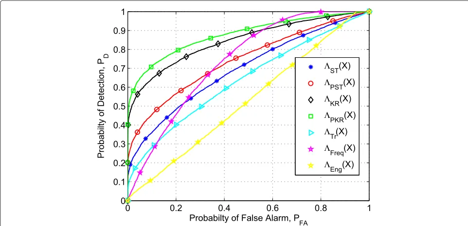
In the first experiment, we obtain the ROC curves using Matlab to compare the performance of the pro-posed schemes to that of the traditional schemes (GLRT that ignores temporal correlation TR(XT), the energy
detectorEng(XT)) and the ST-GLRT and its
frequency-domain approximation for WSS series. In particular, the energy detector can be expressed as:
Eng(XT)=
and the frequency-domain detector is given by (39) in Appendix A. It is to be noted that the energy detector assumes known noise power.
0 0.2 0.4 0.6 0.8 1 0
0.1 0.2 0.3 0.4 0.5 0.6 0.7 0.8 0.9 1
Probabilty of False Alarm, P
FA
Probabilty of Detection, P
D Λ
ST(X) ΛPST(X)
ΛKR(X)
ΛPKR(X)
ΛTr(X)
ΛFreq(X)
ΛEng(X)
Figure 3ROC curves for comparison of detection schemes: sample support sizeM=70, number of vector samples per sub-blockN=10, number of antennasL=4, noise uncertaintyαnu=1, and average SNRκ¯= −10 dB.
setup for the case with noise power uncertainty. Note that we model the noise power uncertainty by generating the
noise power at thel-th antenna asσw2,l∼U
σ2
n,l
αnu,αnuσn2,l
,
where αnu ≥ 1, and αnu = 1 means no noise uncer-tainty [1]. From the results, it is clear that the proposed
schemes clearly outperform traditional schemes. More-over, from the experiment, we can also conclude that the noise power uncertainty slightly deteriorates the per-formance of all detectors. However, the energy detector completely collapses atαnu = 2. To further analyze the effects of the sample support, noise power uncertainty,
0 0.2 0.4 0.6 0.8 1
0 0.1 0.2 0.3 0.4 0.5 0.6 0.7 0.8 0.9 1
Probabilty of False Alarm, P
FA
Probabilty of Detection, P
D
ΛST(X)
ΛPST(X)
ΛKR(X)
ΛPKR(X)
ΛTr(X)
ΛFreq(X)
ΛEng(X)
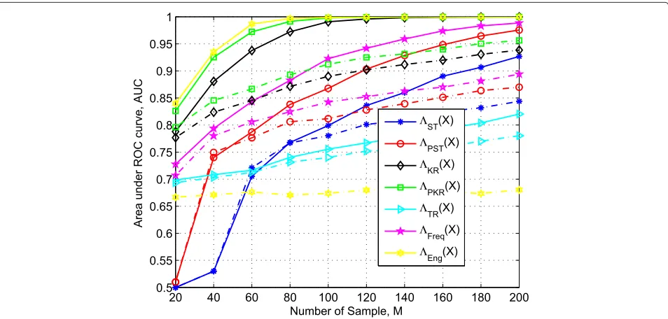
and shadowing parameters, we need to have a single and quantitative figure of merit. This metric is the area under the ROC curve (AUC), which varies between 0.5 (poor performance) and 1 (good performance). Hence, next, we use AUC curves to see effects of the sample sup-port, noise power uncertainty, and shadowing parameters on the detection performance of the spectrum sensing schemes. We model the shadowing effect by using log-normal random variable as:psh = pm10xσ/10, wherepm is the expected signal power at the receiver (equal for all antennas),pshis the signal power after shadowing effect, and xσ is Gaussian random variable with 0 mean and standard deviationσSh. The log-normal shadow fading is often characterized by its dB spread,σdB, which has the relationshipσSh=0.1σdBlog10[38].
In Figure 5, we plot the AUC curves to analyze the effects of sample size in the presence of shadowing, with and without the effects of noise power uncertainty. In this figure, the curves with dashed lines represent the case where both shadowing and noise power uncertainty with αnu = 1.5. On the other hand, the curves with solid lines show the case with no noise power uncertainty (i.e.αnu = 1). From these plots, it can be concluded that the proposed schemes KR(Z) andPKR(Z) are robust against the small sample support both in the presence and absence of noise power uncertainty. Particularly, in the region 20≤M≤80, the detectorsKR(Z)andPKR(Z) clearly outperform the other detectors. As expected, we can also see that in the small sample regime,PKR(Z) per-forms better thanKR(Z). The obvious reason for this is that underH1instead of12L(L+1)+12N(N+1)parameters
in the case of KR(Z), the detection scheme PKR(Z) has approximately only (2L−1)+(2N−1)parameters to estimate. In order to confirm this, in Figure 6, we plot the normalized minimum square error (MSE) of the estimator of the covariance matrix under hypothesisH1, expressed as:
RNMSE=
1
Javg Javg
j=1
ˆj− 2
F 2
F
(38)
where is the true spatio-temporal covariance matrix, ˆ
j is the estimated covariance for each estimator in the Monte Carlo simulationj,.2Fis the Frobenius norm, and Javgis the number of Monte Carlo simulations. The results confirm that for small sample support, estimators of used in the caseKR(Z)andPKR(Z)have smaller error. In Figure 7, we show the AUC plots to analyze the effect of shadowing (i.e. σdB) both in the presence and absence of noise uncertainty, αnu = 1.5 and αnu = 1, respectively. It is clear from these results that the effects of shadowing are very small on the performance of the detection schemes. However, we can see that by incre-mentingσdB, a slight improvement occurs in the perfor-mance of the detection schemes TR(Z), ST(Z), and
PS(Z). The most obvious reason for this interesting outcome can be the heavy-tailed distribution of the pri-mary signal strength due to the log-normally-distributed shadow fading that behaves in such a way at lower SNR [39].
20 40 60 80 100 120 140 160 180 200 0.5
0.55 0.6 0.65 0.7 0.75 0.8 0.85 0.9 0.95 1
Number of Sample, M
Area under ROC curve, AUC
ΛST(X)
ΛPST(X)
ΛKR(X)
ΛPKR(X)
ΛTR(X)
ΛFreq(X)
ΛEng(X)
Figure 5AUC curves (solid lines forαnu=1 and dashed lines forαnu=2) to assess the effects of number of samplesM: number of vector
50
100
150
200
3.2
3.4
3.6
3.8
4
4.2
4.4
Number of Samples, M
Normalized MSE
MLE
Persym−MLE
Kron−MLE
PerKron−MLE
Figure 6Normalized MSE of the estimator of covariance matrix under hypothesisH1.
In Figure 8, we show the AUC plots to analyze the effects of noise power uncertainty. The results show a robust behavior for the detection schemes against the noise power uncertainty. Once again, we observe that the performance of the proposed schemesKR(Z) and
PKR(Z)is better than other schemes that do not exploit the underlying structure of the received signal.
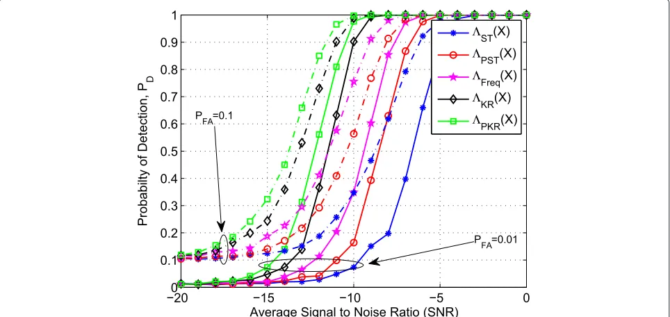
Finally, keeping the probability of false alarmPF fixed, we simulate the performance of the detection schemes by plottingPDagainst different values of average SNRκ¯. The simulation results are shown in Figure 9. The results clearly show that for different SNR values, the proposed schemes consistently perform better than the detection schemes that do not exploit the covariance structure.
0 2 4 6 8 10 12
0.86 0.88 0.9 0.92 0.94 0.96 0.98 1
dB Spread σdB
Area under ROC curve, AUC
ΛST(X)
ΛPST(X)
ΛKR(X)
ΛPKR(X)
ΛTR(X)
1 1.2 1.4 1.6 1.8 2 0.65
0.7 0.75 0.8 0.85 0.9 0.95 1
Noise uncertainty factor, αnu
Area under ROC curve, AUC
ΛST(X)
ΛPST(X)
ΛKR(X)
ΛPKR(X)
ΛTR(X)
ΛFreq(X)
ΛEng(X)
Figure 8AUC curves to assess the effects of noise uncertaintyαnu: with sample sizeM=80, number of vector samples per sub-block N=15, number of antennasL=4, effect of shadowingσdB−spread=4, and average SNRκ¯= −8 dB.
In conclusion, we can say that the exploitation of inher-ent structure of covariance matrix both in frequency and time domain leads us to robustness against the small sample support compared to the ST-GLRT in (9).
6.2 Experiment no. 2: cognitive radio
In the previous set of experiments, we analyzed the pro-posed schemes for detection of a Gaussian signal with
separable spatio-temporal covariance matrix in unknown additive uncorrelated noise. In the present set of exper-iments, we perform simulations to illustrate the appli-cation of the proposed detection schemes in cognitive radio, i.e. with an actual communication signal instead of a Gaussian signal and with a non-separable spatio-temporal covariance matrix. For the simulations, we have used an ODFM-modulated DVB-T signal (8-K mode, 64−QAM,
−200 −15 −10 −5 0
0.1 0.2 0.3 0.4 0.5 0.6 0.7 0.8 0.9 1
Average Signal to Noise Ratio (SNR)
Probabilty of Detection, P
D
ΛST(X)
ΛPST(X)
ΛFreq(X)
ΛKR(X)
ΛPKR(X)
PFA=0.1
P
FA=0.01
0
0.2
0.4
0.6
0.8
1
0
0.2
0.4
0.6
0.8
1
Probability of False Alarm
Probability of Detection
Λ
ST(X)
Λ
PS(X)
Λ
Freq(X)
Λ
KR(X)
Λ
PKR(X)
Λ
Tr(X)
Figure 10ROC curves (solid lines forαnu=2 and dashed lines forαnu=1): sample support sizeM=70, number of vector samples per
sub-blockN=15, number of antennasL=4, channel delay spread 0.779μs, and average SNRκ¯= −8 dB.
guard interval 1/4, and inner code rate 2/3) with a band-width of 7.61 MHz. We have considered a 4×4 Rayleigh channel with unit power and an exponential power delay profile with length 64 samples (at a sampling frequency of 7.61 MHz). The additive noises at each antenna are generated as a zero-mean complex Gaussian process. We used a noise power different at each antenna with average
SNRκ¯ = −8 dB. To analyze the schemes, we plot ROC curves withN = 15 vector samples per sub-block. The rest of the parameters are given in the captions of the figures.
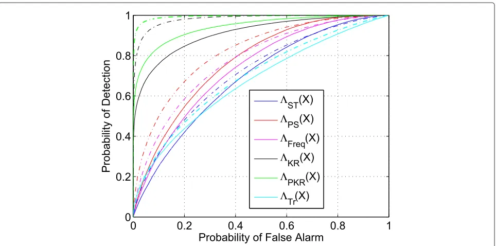
In Figure 10, we plot the ROC curves for the case when the channel delay spread is 0.779 μs with and without noise power uncertainty. In this figure, we can
0
0.2
0.4
0.6
0.8
1
0
0.2
0.4
0.6
0.8
1
Probability of False Alarm
Probability of Detection
Λ
ST(X)
Λ
PS(X)
Λ
Freq(X)
Λ
KR(X)
Λ
PKR(X)
Λ
Tr(X)
Figure 11ROC curves (solid lines forαnu=2 and dashed lines forαnu=1): sample support sizeM=70, number of vector samples per
easily see that the detectorsKR(Z)andPKR(Z)clearly outperform the other detectors, even for this realistic spatio-temporal correlation. In Figure 11, we repeat the experiment of Figure 10 for a channel delay spread 0.097μs (almost flat fading channel). Even for channels with low-frequency selectivity, we can see that the detec-tion schemesKR(Z)andPKR(Z)consistently perform better compared to the rest of the detection schemes. However, compared to Figure 10, in Figure 11, we can see interesting results that the detector which ignores temporal correlation outperforms spatio-temporal correlation-based schemes due to the low selectivity of the channel.
Before commenting on these interesting results, for further confirmation, we need to have a single and quantitative figure of merit, so we plot AUC curves in Figure 12.
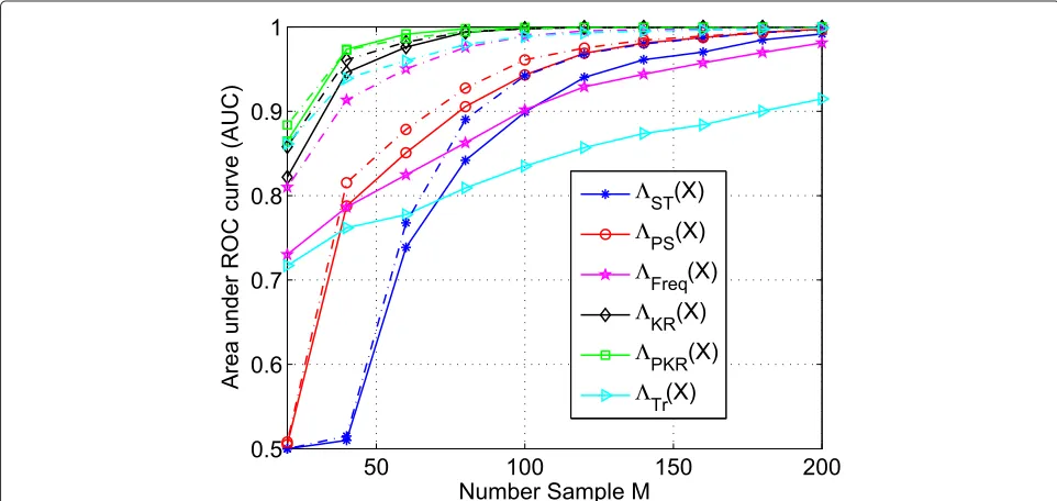
The AUC curves in Figure 12 demonstrate that the proposed detectors have better performance compared to the traditional detection schemes, for different val-ues of sample support. In order to see the effect of delay spreads, we consider two types of channel delay spreads (0.097 and 0.779 μs). The results in Figure 12 confirm that the proposed schemesKR(Z)andPKR(Z) consistently outperform other schemes in small sample support regime. We can also see that in general, the per-formance of all schemes is degraded for different values of delay spreads; since the larger the delay spread, the larger the degradation incurred. However, we can see that compared to rest of the detection schemes,KR(Z)and
PKR(Z) show more robustness against changes in the delay spread. We can further observe an interesting out-come in the case of the detector that ignores temporal correlation and the frequency-based approximate GLRT, where we can see that the performances of these two detection schemes are quite different for the two chan-nel delay spreads. This is also evident from comparison of ROC curves in Figures 10 and 11. The possible expla-nation for this can be that for a short channel delay spread (i.e. 0.097 μs), the multi-tap channel adds neg-ligible temporal correlation. On the other hand, in the case of channel delay spread 0.779μs, we have tempo-ral correlation imposed by the channel on the tempotempo-rally uncorrelated transmitted OFDM signal. Therefore, the inclusion of temporal correlation as an additional detec-tion metric is not helping in the case of delay spread (i.e. 0.097μs).
In order to further analyze the detection performance of the proposed schemes, in Figure 13, we compare the results by plottingPDvs average SNRκ¯. Once again, we can observe that the proposed schemes outperform the remaining detection schemes presented in this paper.
7 Conclusion
In this paper, we have proposed novel detection schemes that exploit the spatio-temporal correlation present in the received observations at a multi-antenna receiver. When exploiting the spatio-temporal correlation, we have observed that the GLRT performs poorly when the sam-ple support is small. To cope with this problem, we
50 100 150 200
0.5 0.6 0.7 0.8 0.9 1
Number Sample M
Area under ROC curve (AUC)
ΛST(X)
ΛPS(X)
ΛFreq(X)
ΛKR(X)
ΛPKR(X)
ΛTr(X)
−120 −10 −8 −6 −4 −2 0 0.1
0.2 0.3 0.4 0.5 0.6 0.7 0.8 0.9 1
Average Signal to Noise Ratio (SNR)
Probabilty of Detection, P
D
ΛST(Z)
ΛFreq ΛKR ΛPKR P
FA=0.1
P
FA=0−01
Figure 13PDvs average SNR: number of vector samples per sub-blockN=15, number of antennasL=4,M=80, channel delay spread
0.097μs.
have proposed detectors that are robust against the sample support. The proposed detectors (approximately) exploit the inherent spatio-temporal structure of the received covariance matrix by using the properties of persymmetric matrices and the Kronecker product of the spatial and temporal covariance matrices. The per-formance of the proposed detectors has been evaluated with the help of numerical simulations, which show important improvements compared to the traditional schemes.
Endnotes
aWe begin with the complex base-band signal sampled
at the specific Nyquist rate.
bThese values are maintained during Monte-Carlo
process. In order to create noise power uncertainty, these values are affected by random uncertainty at each run.
Appendix
A Approximated GLRT in the frequency domain
For the interested readers, herein, we reproduce the approximated GLRT in the frequency domain, originally presented in [15]. While considering the case in which the received signals are jointly WSS, the limiting form (Lfixed and M,N → ∞) of the the frequency domain GLRT statistic is written as [15]:
ST
Zf −→ M,N→∞exp
⎧ ⎨ ⎩
π
−πlog ⎡ ⎣det
ˆ Sejθn
!L i=1sˆii
ejθn
⎤ ⎦dθn
2π
⎫ ⎬ ⎭,
(39)
where Sˆejθn
l,k = f
Hejθn ˆ
l,kf
ejθn is a quadratic estimator and the Fourier vector is given by
fejθn =1,e−jθn,e−j2θn,e−j3θn,. . .,e−j(N−1)θnT. (40)
Competing interests
The authors declare that they have no competing interests.
Acknowledgements
This work was supported by the Catalan Government under the grant FIDGR- 2011-FIB0071.
Author details
1SPCOMNAV, Universitat Autònoma de Barcelona, 08193 Bellaterra, Barcelona, Spain.2Electrical Engineering, University of Engineering and Technology, Peshawar, 25000 Peshawar, Pakistan.3Department of Electrical Engineering and Information Technology (EIM-E), Universität Paderborn, Paderborn, Germany.4Signal Processing School of Electrical Engineering, KTH Royal Institute of Technology, SE-100 44 Stockholm, Sweden.
Received: 1 July 2014 Accepted: 25 October 2014 Published: 7 November 2014
References
1. E Biglieri, AJ Goldsmith, LJ Greenstein, NB Mandayam, HV Poor,Principles of Cognitive Radio(Cambridge University Press, Cambridge, 2012) 2. AW Min, X Zhang, KG Shin, Detection of small-scale primary users in
cognitive radio networks. IEEE J. Selected Areas Commun.29, 349–361 (2011)
3. R Zhang, TJ Lim, Y-C Liang, Y Zeng, Multi-antenna based spectrum sensing for cognitive radios: a GLRT approach. IEEE Trans. Commun. 58(1), 84–88 (2010)
5. Y Zeng, Y-C Liang, AT Hoang, R Zhang, A review on spectrum sensing for cognitive radio: challenges and solutions. EURASIP J. Adv. Signal Process. (2010). doi:10.1155/2010/381465
6. W Yang, G Durisiand, VI Morgenshtern, E Riegler, inProc. ISWCS. Capacity pre-log of SIMO correlated block-fading channels (Piscataway, 2011), pp. 869–873
7. KV Mardia, JT Kent, JM Bibby,Multivariate Analysis, 1st edn. (Academic Press, Waltham, 1979), p. 536
8. TW Anderson,An Introduction to Multivariate Statistical Analysis
(Wiley-Interscience, Hoboken, 2003)
9. Y Zeng, Y-C Liang, Eigenvalue-based spectrum sensing algorithms for cognitive radio. IEEE Trans. Commun.57(6), 1784–1793 (2009) 10. C Vazquez-Vilar, R López-Valcarce, Spectrum sensing exploiting guard
bands and weak channels. IEEE Trans. Signal Process.59(12), 6045–6057 (2011)
11. Z Quan, W Zhang, SJ Shellhammer, A Sayed, Optimal spectral feature detection for spectrum sensing at very low SNR. IEEE Trans. Commun. 59(1), 201–212 (2011)
12. J Sala-Alvarez, G Vazquez-Vilar, R Lopez-Valcarce, Multiantenna GLR detection of rank-one signals with known power spectrum in white noise with unknown spatial correlation. IEEE Trans. Signal Process. 60(6), 3065–3078 (2012)
13. A Perez-Neira, M-A Lagunas, MA Rojas, P Stoica, Correlation matching approach for spectrum sensing in open spectrum communications. IEEE Trans. Signal Process.57(12), 4823–4836 (2009)
14. G Vazquez-Vilar, R Lopez-Valcarce, J Sala, Multiantenna spectrum sensing exploiting spectral a priori information. IEEE Trans. Wireless Commun. 10(12), 4345–4355 (2011)
15. D Ramirez, J Via, I Santamaria, LL Scharf, Detection of Spatially Correlated Gaussian Time Series. IEEE Trans. Signal Process.58(10), 5006–5015 (2010) 16. TF Ayoub, AR Haimovich, Modified GLRT signal detection algorithm.
IEEE Trans. Aerospace Electron. Syst.36(3), 810–818 (2000)
17. Y Chen, A Wiesel, AO Hero, inProc. of IEEE ICASSP. Shrinkage Estimation of High Dimensional Covariance Matrices (Piscataway, 2009), pp. 2937–2940 18. D Ramírez, G Vazquez-Vilar, R López-Valcarce, J Vía, I Santamaría,
Detection of rank-p signals in cognitive radio networks with uncalibrated multiple antennas. IEEE Trans. Signal Process.59(8), 3764–3774 (2011) 19. R Nitzberg, Application of maximum likelihood estimation of
persymmetric covariance matrices to adaptive processing. IEEE Trans. Aerospace Electron. Syst.16(1), 124–127 (1980)
20. D Akdemir, AK Gupta, Array variate random variables with multiway Kronecker delta covariance matrix structure. J. Algebraic Stat.2(1), 98–113 (2011)
21. P Wirfalt, M Jansson, inProc. of Sensor Array and Multichannel Signal Processing Workshop (SAM). On Toeplitz and Kronecker Structured Covariance Matrix Estimation (Piscataway, 2010), pp. 185–188
22. K Werner, M Jansson, P Stoica, On estimation of covariance matrices with Kronecker product structure. IEEE Trans. Signal Process.56(2), 478–491 (2008)
23. N Lu, DL Zimmerman, The likelihood ratio test for a separable covariance matrix. Stat. Probab. Lett.73(5), 449–457 (2005)
24. MG Genton, Separable approximations of space-time covariance matrices. Environmetrics18(7), 681–695 (2007)
25. S Ali, JA López-Salcedo, G Seco-Granados, inProc. of 20th European Signal Processing Conference. Exploiting Structure of Spatio-temporal Correlation for Detection in Wireless Sensor Networks (Piscataway, 2012), pp. 774–778
26. Y Liang, VV Veeravalli, Capacity of noncoherent time-selective rayleigh-fading channels. IEEE Trans. Inform. Theory50(12), 3095–3110 (2004)
27. SM Kay,Fundamentals of Statistical Signal Processing, Volume 2: Detection Theory(Prentice Hall, Upper Saddle River, 1998)
28. L Lu, H-C Wu, SS Iyengar, A novel robust detection algorithm for spectrum sensing. IEEE J. Selected Areas Commun.29(2), 305–315 (2011) 29. M Wax, T Kailath, Efficient inversion of Toeplitz-block Toeplitz matrix.
IEEE Trans. Acoustics, Speech Signal Process.31(5), 1218–1221 (1983) 30. J Ward,Space-Time Adaptive Processing for Airborne Radar.Technical
Report 1015, Lincoln Laboratory, MIT, (Lexington, December 1994) 31. TK Huckle, K Waldherr, T Schulte-Herbrüggen, Exploiting matrix
symmetries and physical symmetries in matrix product states and tensor trains. Linear Multilinear Algebra61(1), 91–122 (2013)
32. M Jansson, P Stoica, Forward-only and forward-backward sample covariances – a comparative study. Signal Process.77(3), 235–245 (1999) 33. B Armour, Structured Covariance Autoregressive Parameter Estimation.
PhD thesis, Department of Electrical Engineering, McGill Canada, 1989 34. J Kamm, J Nagy, Optimal Kronecker Product Approximation of Block
Toeplitz Matrices. SIAM J. Matrix Anal. Appl.22(1), 155–172 (2000) 35. MW Mitchell, MG Genton, ML Gumpertz, A likelihood ratio test for separability of covariances. J. Multivar. Anal.97(5), 1025–1043 (2006) 36. P Dutilleul, The MLE algorithm for the matrix normal distribution. J. Stat.
Comput. Simul.64, 105–123 (1999)
37. T Fawcett,ROC graphs: Notes and practical considerations for researchers.
Technical Report HPL-2003-4, HP Laboratories, (Palo Alto, 2003) 38. A Ghasemi, ES Souca, Asymptotic performance of collaborative spectrum
sensing under correlated log-normal shadowing. IEEE Commun. Lett. 11(1), 34–36 (2007)
39. T Muetze, P Stuedi, F Kuhn, G Alonso, inProc. of IEEE SECON,San Francisco. Understanding radio irregularity in wireless networks (Piscataway, 2008), pp. 82–90
doi:10.1186/1687-6180-2014-160
Cite this article as:Aliet al.:Multi-antenna spectrum sensing by exploiting spatio-temporal correlation.EURASIP Journal on Advances in Signal Processing20142014:160.
Submit your manuscript to a
journal and benefi t from:
7Convenient online submission 7Rigorous peer review
7Immediate publication on acceptance 7Open access: articles freely available online 7High visibility within the fi eld
7Retaining the copyright to your article