Statistical monitoring of aftershock sequences: a case study of the 2015 Mw7 8 Gorkha, Nepal, earthquake

LETTER

Statistical monitoring of aftershock

sequences: a case study of the 2015 Mw7.8

Gorkha, Nepal, earthquake

Yosihiko Ogata

_{and Hiroshi Tsuruoka}

Abstract

Early forecasting of aftershocks has become realistic and practical because of real-time detection of hypocenters. This study illustrates a statistical procedure for monitoring aftershock sequences to detect anomalies to increase the prob-ability gain of a significantly large aftershock or even an earthquake larger than the main shock. In particular, a signifi-cant lowering (relative quiescence) in aftershock activity below the level predicted by the Omori–Utsu formula or the epidemic-type aftershock sequence model is sometimes followed by a large earthquake in a neighboring region. As an example, we detected significant lowering relative to the modeled rate after approximately 1.7 days after the main shock in the aftershock sequence of the Mw7.8 Gorkha, Nepal, earthquake of April 25, 2015. The relative quiescence lasted until the May 12, 2015, M7.3 Kodari earthquake that occurred at the eastern end of the primary aftershock zone. Space–time plots including the transformed time can indicate the local places where aftershock activity lowers (the seismicity shadow). Thus, the relative quiescence can be hypothesized to be related to stress shadowing caused by probable slow slips. In addition, the aftershock productivity of the M7.3 Kodari earthquake is approximately twice as large as that of the M7.8 main shock.

Keywords: Epidemic-type aftershock sequence (ETAS) model, Omori–Utsu formula, Change-point, Probability gain, GUI software package XETAS, Relative quiescence, Seismicity shadow

© 2016 Ogata and Tsuruoka. This article is distributed under the terms of the Creative Commons Attribution 4.0 International License (http://creativecommons.org/licenses/by/4.0/), which permits unrestricted use, distribution, and reproduction in any medium, provided you give appropriate credit to the original author(s) and the source, provide a link to the Creative Commons license, and indicate if changes were made.

Background

On April 25, 2015, a strong earthquake of Mw7.8 occurred along the Himalayan front close to Kathmandu, Nepal. Seventeen days after the main shock, the larg-est aftershock of May 12, the M7.3 Kodari earthquake, occurred in the eastern extension of the primary after-shock zone. The dip angle of the rupture fault zone is similar to that of the main fault zone on the plate bound-ary between the Indian and Eurasian plates.

The global probability forecast of the aftershocks of this earthquake (Michael et al. 2015) was implemented on the basis of near-real-time data of the National Earthquake Information Center (NEIC), refer to Page et  al. (2015) for the method and procedure for the near-real-time

global forecast. The initial forecast used the Reasen-berg and Jones (1989) model with generic parameters of the region, which combine the Omori–Utsu law for the decay of aftershock frequency (Omori 1894; Utsu

1961) and the Gutenberg–Richter law for magnitude fre-quency (Gutenberg and Richter 1944). The model was subsequently updated to reflect a lower productivity and higher decay rate based on the observed aftershocks. This proved to be consistent with the main topic addressed in this paper. In fact, the forecast of the size distribution of aftershocks due to the Reasenberg–Jones predictor assumes the Gutenberg–Richter law. However, when pre-cursory anomalies that can raise the probability gain of a large earthquake were detected, the probability forecast of the M7.3 aftershock was significantly small using this predictor only.

Retrospectively, we think that the forecast in this case could have yielded a higher likelihood of large-magnitude aftershocks than that predicted under the

Open Access

*Correspondence: ogata@ism.ac.jp

1 _{The Institute of Statistical Mathematics, 10-3 Midori-cho, Tachikawa,} Tokyo 190-8562, Japan

Gutenberg–Richter law. Relevant to this issue, Utsu (1979) and Aki (1981) emphasized the role of seismic anomalies in predicting the enhancement of the likeli-hood (probability gain) of having a substantially larger earthquake than the secular probability of the same size of earthquake. After the appearance of an anomaly, we need to evaluate the probability that it will be a precursor to a large earthquake; i.e., we need to forecast whether the probability in a space–time zone will increase to an extent, relative to that of the reference probability. Hence, it is desirable to search for anomalous phenomena that enhance the probability gains.

Seismic quiescence has attracted attention as a pre-cursor candidate of large earthquakes (Inouye 1965; Utsu 1968; Ohtake et al. 1977; Wyss and Burford 1987; Kisslinger 1988). This anomaly concept is extended to include aftershock activity that can be significantly lower than the prediction of the Omori–Utsu formula (Matsu’ura 1986) or than the epidemic-type after-shock sequence model (ETAS model; Ogata 1988, 1992,

2001a, for example). The quiescence relative to the ETAS model is useful for the detailed description of aftershock sequences as well as general seismicity. Development of the statistical models and analysis methods of aftershock sequences can be found in Utsu et al. (1995).

From comprehensive study, the retrospective statisti-cal results from Japanese data (Ogata 2001a) suggest that the probability gain of having another large earthquake of a similar size to the main shock becomes several times greater relative to the normal probability if the aftershock activity shows significant lowering. Therefore, it is nec-essary to pay careful attention to anomalous activity by monitoring the aftershock sequence, especially in the early stage.

Methods

Statistical models to monitor aftershock sequences

Short-term probability prediction of an earthquake of magnitude Mz or larger in a near-future period (t, t + dt) is given by _θ(t|Ht)dt where _θ(t|Ht) is the history-dependent occurrence rate, for example, the ETAS model developed by Ogata (1985, 1988, 1989)

where t =  0 is the main shock time of the aftershock observation and Mz represents the reference magnitude (i.e., the main shock magnitude) of earthquakes to be treated in the dataset. Mi and ti indicate the magnitude and the occurrence time of the ith earthquake, respec-tively, and Ht represents the occurrence series of earth-quakes (ti, Mi) before time t. The parameter set θ thus

term of Eq. (1) is a weighted superposition of the Omori– Utsu empirical function (Utsu 1961) for aftershock decay rates;

where t is the elapsed time from the occurrence of a main shock.

These parameters are obtained by maximizing the log-likelihood function (Ogata 1983, 1988, 1989) with respect to the parameter set θ. The log-likelihood function of the ETAS model,

is maximized with respect to the parameter set θ = (µ, K, c, α, p). Here, ‘ln’ is a natural logarithm, and {(ti, Mi), Mi ≥ Mc; i = 1, 2, …} are occurrence times and magni-tudes of earthquakes in the target time interval [S, T] for the fitting. Note here that the fitted data in the target interval [S, T] do not contain the main shock and imme-diately following aftershocks during the period [0, S), but that _θ(t|Ht) include the data of the main shock and aftershocks during the period [0, S) as the preceding his-tory. Note also that the Omori–Utsu model is not history dependent except for the elapsed time since the main shock, and it is possible to apply the same log-likelihood function as (3) with θ = (K, c, p). The obtained param-eter values are called the maximum likelihood estimates (MLE).

The Reasenberg and Jones method combines the Omori–Utsu aftershock decay, Utsu productivity scal-ing (Utsu 1970), and Gutenberg–Richter magnitude distribution (Gutenberg and Richter 1944), such that _(t)·10−b(M−Mc)_{. Similarly, (t|Ht)·10}−b(M−Mc) _can yield a better forecast for the case of multiple sources of earthquake clustering.

In terms of prediction, the goodness of fit of the model is measured using the Akaike information criterion (AIC; Akaike 1973), which is described as

where ln L(θ) represents the log likelihood (3) of the sta-tistical model and k is the number of parameters to be estimated. With this criterion, the model with a smaller value of the AIC is expected to perform better predic-tion. The difference in the AIC values, ΔAIC, between the two competing models is useful, because exp{−

et al. 1998). Hence, for an aftershock sequence, a simpler model with a smaller number of adjusted parameters will yield a smaller AIC value if the difference in the maxi-mum log-likelihood values is smaller than 1.0. Therefore, we may sometimes assume fixed parameter values μ = 0 or generic parameters such as p = 1.0 in the aftershock sequence to compare the AIC value of the ETAS model or the Omori–Utsu model.

When a seismicity change is suspected, we may look at the most likely candidate for the change-point time T0 in a given period [S, T]. First, we separately fit

suit-able statistical models for the divided periods [S, T0] and

[T0, T] (two-stage model), and then we compare their

total performance against the model fitted over the whole period [S, T] by the AIC. Then the most likely estimate of change-point should minimize

or maximize the likelihood (e.g., Bansal and Ogata 2013)

with respect to the change-point candidate parameter T0,

which can be called the MLE of the change-point with respect to the time.

Theoretical cumulative function and time transformation Suppose that the parameter values θ = (μ, K, c, α, p) of the ETAS model (1) are given. Then the integral of the conditional intensity function,

provides the expected cumulative number of earthquakes in the time interval [S, t]. The time transformation from t to τ is considered based on this cumulative intensity;

transforms the ordinary occurrence times of aftershocks; (t1, t2, …, tN) into the sequence (τ1, τ2, …, τN) in the time interval [0, Λ(T)], which we call the residual point process (RPP). If the model is a good approximation to the real seis-micity, we expect its integrated function (7) and the empiri-cal cumulative counts N(t) of the observed earthquakes to be similar to each other. This implies that the transformed sequence (the RPP) appears to be a stationary Poisson pro-cess (uniformly distributed occurrence times) with unit intensity (occurrence rate) if the model is sufficiently cor-rect, but it appears to be heterogeneous otherwise.

Let N(σ, τ) be the number of events in the interval (σ, τ) in the transformed time axis. If no change in after-shock activity occurs, the extrapolated RPP is also the standard stationary Poisson process with the same unit intensity, and the deviation N(τ0, τ )−(τ−τ0) of the

empirical cumulative function is approximately dis-tributed according to the normal distribution N_{(0,�τ )} where Δτ = τ − τ0. However, when the number of events N(σ, τ0) in the target interval (σ,τ0) is not large enough,

the significance actually depends on the sample size, due to the estimation accuracy of the parameters for the transformation. Thus, taking such accuracy into consid-eration, the error distribution of �N(τ0,τ ) is modified

to be N

0, �τ +(�τ )2/N(σ,τ0), derivation of which is provided in Appendix B of Ogata (1992). Hereafter we define the anomaly in the case where the empiri-cal cumulative function deviates outside the parabola of 95 % significance 2

�τ+(�τ )2/N(σ,τ0)

.

The FORTRAN program package associated with man-uals regarding the ETAS analysis is available to calculate the MLE of θ and also to visualize model performances (Ogata 2006c), which has been extended to the program package XETAS (Tsuruoka and Ogata 2015a, b) using graphical user interface (GUI).

Data and results

We first used the NEIC Preliminary Determination of Epicenters (PDE) for datasets of the on-fault aftershocks in the rectangular area bounded by the 84.4°E and 86.4°E meridians and 27.2°N and 28.4°N parallels obtained on May 13, 2015 (the day after the M7.3 Kodari earthquake; hereafter termed the first PDE data). Results similar to those of this study using this dataset were reported in early June 2015 at a workshop (Ogata 2015; Tsuruoka and Ogata 2015a). In addition, we used the second PDE data obtained on July 22, 2015 (Tsuruoka and Ogata 2015b), and herein we also incorporate the final datasets from the Advance National Seismic Network (ANSS) obtained on October 31, 2015.

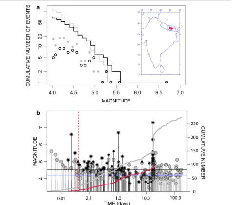
We used the TSEIS visualization program pack-age (Tsuruoka 1996) for selection of datasets from the catalogs. The identified aftershocks in the PDE catalog increase as time evolves, and the ANSS catalog includes about twice as many primary aftershocks before the M7.3 event as the first PDE data. In addition to the relo-cated epicenters and re-evaluated magnitudes of the same aftershocks, newly detected aftershocks are listed as time proceeds. Figure 1a, b shows such differences between the first PDE data and the ANSS data; as far as the sequences of occurrence times and magnitudes are concerned, the second PDE data and the ANSS data are almost identical.

We use the GUI program package XETAS (Tsuruoka and Ogata 2015a, b), efficiently implementing the above-mentioned methods in the following statistical analysis. The estimation results are summarized in Table 1.

occurrence time of the largest aftershock of M7.3. The threshold magnitude is taken as M4.5 for complete-ness in the period from 1 h after the main shock occur-rence time, as shown in Fig. 1. We apply the ETAS model and the Omori–Utsu model to this entire period. Table 1a indicates that the ETAS model fits better than the Omori–Utsu model according to the AIC values. The estimated decaying parameter p values of both the

Omori–Utsu and ETAS models are seemingly quite large; this may be explained as follows.

By applying the ETAS model to the dataset for a whole target period, we preliminarily search a time interval in which change-points seem to exist, inspecting the devia-tions of the cumulative curve of the transformed time (8) from the straight line. We then calculate exp(−ΔAIC/2) of the likelihood of change-point time (see “Methods”

Fig. 1 Detected aftershocks and their magnitudes. aOpen circles and gray dots indicate the frequencies of identified aftershocks against magni-tudes for the period between the main shock and the M7.3 largest aftershock, listed in the PDE catalog at May 13, 2015, and the ANSS catalog at October 31, 2015, respectively. The black and gray step functions are the cumulative numbers of identified aftershocks from the largest magnitude to the lowest, corresponding to the magnitude frequencies. b Magnitude versus elapsed time from the main shock on a logarithmic scale. Black

section above). Thus, as given in Table 1, the 1.7  days from the main shock occurrence are the most likely (MLE) candidate of change-point time. Incidentally, we cannot detect a significant local peak around the time (1.04 days) of the second largest aftershock of M6.7.

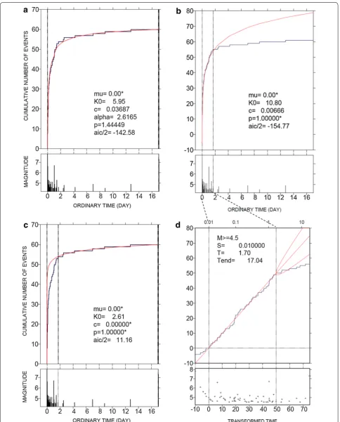
After the MLE of the change-point, the number of after-shocks of M4.5 and larger become markedly low, so we suspect that there was a change in the seismicity pattern at the time. According to Table 1a, the Omori–Utsu model with very high p value fits better than the ETAS model in the period from 1  h until the suspected change-point time (1.7 days) before the M7.3 aftershock. The difference in the AIC/2 values is small, and thus the simpler model is preferred for the prediction, probably due to the small number of events at this threshold magnitude. Figure 2a–c shows the best-fit models for the entire period (ETAS) and for the separate periods (the Omori–Utsu model and

stationary Poisson model). Figure 2b, d shows the fit of the Omori–Utsu cumulative curve to the empirical cumula-tive function before the change-point at 1.7 days after the main shock and also show the deviation from the empirical cumulative function after the change-point. These show that about 20 potentially expected aftershocks of M4.5 or larger did not occur during the quiet period.

Next, to examine the stability of the above results, we also use the ANSS data for similar analysis of the after-shocks before the M7.3 event for various target periods and lower threshold magnitudes as described in Table 1b to ensure completeness of the datasets in accordance with Fig. 1. In these data from the ANSS catalog, the likely change-point estimate is also 1.7 days. The results of the O–U and the ETAS models are similar to each other according to Table 1b. For the primary aftershocks throughout the entire period until the M7.3 event, the

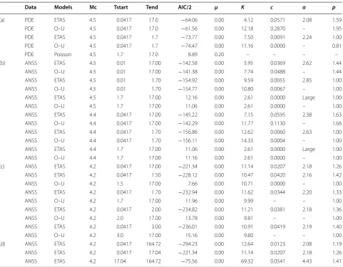
Table 1 MLE of the models and values of the AIC/2 for respective datasets

‘Tstart’ and ‘Tend’ indicate the range of target intervals of respective datasets. ‘O–U’ is an abbreviation for the Omori–Utsu model. Blocks (a)–(d) provide the fitted results of the models for the same datasets but different setups, as cited in the text

Data Models Mc Tstart Tend AIC/2 μ K c α p

(a) PDE ETAS 4.5 0.0417 17.0 −64.06 0.00 4.12 0.0571 2.08 1.59 PDE O–U 4.5 0.0417 17.0 −61.56 0.00 12.18 0.2870 – 1.95 PDE ETAS 4.5 0.0417 1.7 −73.77 0.00 7.50 0.0091 2.24 1.00 PDE O–U 4.5 0.0417 1.7 −74.47 0.00 11.16 0.0000 – 0.81

PDE Poisson 4.5 1.7 17.0 8.89 0.20 – – – –

(b) ANSS ETAS 4.5 0.01 17.00 −142.58 0.00 5.95 0.0369 2.62 1.44 ANSS O–U 4.5 0.01 17.00 −141.38 0.00 7.74 0.0488 – 1.44

ANSS ETAS 4.5 0.01 1.70 −154.92 0.00 9.59 0.0055 2.85 1.00

ANSS O–U 4.5 0.01 1.70 −154.77 0.00 10.80 0.0067 – 1.00

ANSS ETAS 4.5 1.7 17.00 12.16 0.00 2.61 0.0000 Large 1.00 ANSS O–U 4.5 1.7 17.00 11.06 0.00 2.61 0.0000 – 1.00 ANSS ETAS 4.4 0.0417 17.00 −145.22 0.00 7.15 0.0595 2.38 1.63 ANSS O–U 4.4 0.0417 17.00 −142.29 0.00 11.77 0.1130 – 1.68 ANSS ETAS 4.4 0.0417 1.70 −156.86 0.00 12.62 0.0060 2.63 1.00 ANSS O–U 4.4 0.0417 1.70 −156.11 0.00 14.33 0.0004 – 1.00 ANSS ETAS 4.4 1.7 17.00 11.06 0.00 2.61 0.0000 Large 1.00 ANSS O–U 4.4 1.7 17.00 11.16 0.00 2.61 0.0000 – 1.00 (c) ANSS ETAS 4.2 0.0417 17.00 −221.34 0.00 11.14 0.0207 2.18 1.26 ANSS ETAS 4.2 0.0417 1.50 −228.12 0.00 10.47 0.0420 2.16 1.42 ANSS O–U 4.2 1.5 17.00 7.66 0.00 10.71 0.0000 – 1.00 ANSS ETAS 4.2 0.0417 1.70 −232.94 0.00 11.62 0.0344 2.20 1.33

ANSS O–U 4.2 1.7 17.00 11.96 0.00 9.99 – – 1.00

ANSS ETAS 4.2 0.0417 2.00 −234.82 0.00 11.21 0.0381 2.18 1.36

ANSS O–U 4.2 2.0 17.00 13.78 0.00 9.81 – – 1.00

ANSS ETAS 4.2 0.0417 3.00 −236.01 0.00 10.91 0.0419 2.19 1.40

ANSS O–U 4.2 3.0 17.00 15.16 0.00 9.80 – – 1.00

ETAS model fits better than the Omori–Utsu model, and the p values of the both models are rather high, namely 1.4–1.7. In the target period before the suspected change-point, the ETAS model shows a slightly better fit than the Omori–Utsu model, possibly because of the increased data size, but the p values of the both mod-els remain generic, namely p = 1.0 in this case. Figure 3

shows the case where the target interval is from 0.01 days (approximately 15 min) until the suspected change-point at 1.7 days and with a threshold magnitude of M4.5. Rela-tive quiescence is also likely to have occurred. Figure 3b, d also shows that about 20 potentially expected after-shocks of M4.5 or larger did not occur during the quiet period.

We further examined aftershocks from the ANSS cat-alog with the possible lowest homogeneous threshold magnitude of M = 4.2 in the period from 1 h until the M7.3 event, in accordance with Fig. 1. The most likely change-point candidate in this case is 2.0 elapsed days as given in Table 1c, but Fig. 4a, b shows that the after-shock activity after day 2 until the M7.3 event appears to have decayed normally as predicted. Hence, we may con-clude that aftershock activity with M ≥ 4.2 was normal throughout the entire period before the M7.3 event.

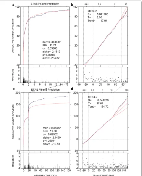
We examine whether any seismicity change occurred after the M7.3 event. The results of the ETAS fitting are given in Table 1d, and Fig. 4c, d shows that second-ary aftershocks of M ≥  4.2 occurred significantly more often than predicted. From the plot of magnitude versus transformed time in Fig. 4d, there are a substantial num-ber of missing aftershocks of M ≥ 4.2 immediately after the M7.3 event. Hence, the actual number of secondary aftershocks was about twice as large as that predicted from the primary aftershock activity, and the aftershock productivity of the M7.3 event was twice as large as that of the main shock of M7.8. This finding implies that a sin-gle ETAS model does not always provide a proper fore-cast of the secondary aftershock sequence from the fit of the primary aftershock sequence, as illustrated in Fig. 4. This is because the ETAS model assumes the same pro-ductivity coefficient for every earthquake, but this is not always true in real seismicity (cf. Ogata 2001b).

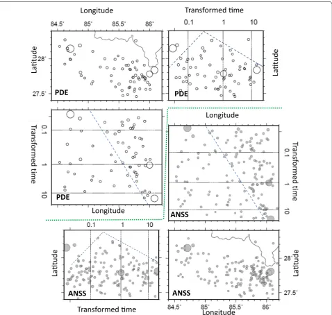
It is also worthwhile to assess the space–time evolu-tion of aftershock occurrences in Fig. 5 with respect to the transformed time using the Omori–Utsu cumula-tive curves. Although the detection rate of smaller after-shocks gradually increased with elapsed time, we used all the located aftershocks in both the near-real-time PDE catalog and the ANSS catalog and fitted the Omori–Utsu model to them to obtain detrended space–time after-shock occurrences with respect to transformed time. Here, we should note that such space–time occurrence is not always uniform with respect to the transformed time

at any place, and nonuniform occurrence times of after-shock activity are often observed in some local regions with respect to the transformed time, such as transient lowering or activation (Ogata 2010a).

On the basis of the space–time plots of aftershocks from both catalogs including the transformed time until the M7.3 event in Fig. 5, we can conclude that the spatial distribution of the primary aftershocks was heterogene-ous, as detailed below.

The plots of epicenter longitudes against transformed times indicate that the eastern part of the aftershock zone was more active than the western part, which includes the main shock; and the western sparser area of after-shocks expanded toward the east. In the shrinking active eastern zone, the M6.7 large aftershock occurred on April 26 (approximately 1 day after the main shock), and then the active zone became quiet until the appearance of densely populated smaller aftershocks near the location of the M7.3 event around 86.1°E. Relevantly, Matsu’ura (1986) commented that relative quiescence is probably activated just before large aftershocks; hence, these may represent some type of foreshocks of a large aftershock.

The plot of epicenter latitudes against transformed times in Fig. 5 indicates that the early aftershocks near the main shock were very sparse but recovered to some extent in about a day. This result suggests that triggering of aftershocks around the main shock was delayed. Then the northern region become quiet and also shows expan-sion toward the eastern end near the Kodari earthquake of M7.3.

Discussion

Seismicity quiescence and empirical medium‑term forecasting

Although quite a number of years have passed since seis-mologists said that seismic quiescence could be effec-tive in prediction, there have not been many examples of quiescence that have been pointed out in advance of a major earthquake. Also, the number and conditions of the parameters that describe the involved relation-ship between the space–time domain of quiescence and potential large earthquakes for general seismic activity are too large to yield a definite answer.

Fig. 4 Overall activity of aftershocks of M ≥ 4.2. Empirical (black) and theoretical (red) cumulative functions and magnitudes plotted against ordi-nary time (a, c) and transformed times (b, d). a, b The ETAS fitting in the target interval from 1 h until 2 days and then extrapolated until the M7.3 event; c, d The ETAS fitting in the target interval from 1 h until the M7.3 event and then extrapolated until the end of October 2015. The parabolas in

aftershocks are attenuated as expected by the model, we empirically expect a higher possibility of a significantly large aftershock, which will probably occur on a fault boundary.

This type of empirical probability gain has been obtained in a large number of case studies. For example, Ogata (2001a) investigated 76 aftershock

sequences in Japan, detected relative quiescence in 34 cases, and evaluated the probability gain of a large earthquake as follows. First, if a large earthquake has occurred in a particular location, the probability per unit area that another earthquake of similar magni-tude will occur in the vicinity is greater than the prob-ability for a distant area. This is the result of empirical

Longitude

Latude

Latude

Longitude

PDE

ANSS

Transformed me

Transformed me

_Longitude

Latude

Latude

Longitude

PDE

PDE

ANSS

ANSS

statistics regarding the self-similarity feature (inverse-power law correlations) and also physically suggests that the neighboring earthquake will be more likely to be induced by a sudden stress change on the periphery because of the abrupt slip of the earthquake. Moreo-ver, if aftershock activity becomes relatively quiet, it becomes more likely that large aftershocks will occur around the boundary of the aftershock area. Further-more, if relative quiescence lasts for a sufficiently long time (more than a few months), the probability of another earthquake of similar magnitude will increase to about three times the probability gain within 6 years in the vicinity of the aftershock area (within 200  km distance). Similar evaluations may be carried out to obtain the probability gain for an aftershock that is larger than magnitude M0 −  0.5 for a main shock of

magnitude M0, for example, in a shorter period of

rela-tive quiescence.

If the detection rates of aftershocks regarding mag-nitudes are same throughout the target period, we can make use of a homogeneous dataset under a smaller threshold magnitude instead of the dataset of completely detected threshold magnitudes to allow less-uncertain inference and prediction (Ogata and Katsura 1993, 2006). It is also desirable to recover information on missing aftershocks using modeling of detection rates, particu-larly in the early stage of aftershocks (Omi et  al. 2013,

2014a, b).

The physical meaning of seismic quiescence

When a significant quiescence has been detected, it is necessary to question whether and how this leads to large earthquakes, if any occur. There are various conditions such as tectonics and stress fields that can be used for quantitative representation of the quiescence phenom-enon to be addressed. A comprehensive physical study of the seismic quiescence preceding a large earthquake is essential for enhancement of the probability gain of the anomaly. These elements must be incorporated to achieve a predicted probability that exceeds the predic-tions of typical statistical models. Specifically, using the model, some retrospective case studies (Ogata 2013; and references therein) have been concerned with the phe-nomenon that the stress shadow (e.g., Harris 1998) inhib-its normal aftershock activity.

As discussed in Ogata (2005a, b, c, 2006a, b, 2007,

2010b, 2011), Ogata et al. (2003), Kumazawa et al. (2010), and Kumazawa and Ogata (2013), we should consider and demonstrate the relationship of seismicity lower-ing (seismicity shadow) in the space–time aftershock occurrence patterns together with slow slips on the plate boundary using geodetic studies for the present Gorkha case (e.g., Avouac et al. 2015; Zhang et al. 2015; Fielding

et  al. 2015; Grandin 2015; Ingleby et  al. 2015). Specifi-cally, scenarios explaining the relative quiescence can rely on the seismicity rate change based on the rate-and-state friction law of Dieterich (1994) as the quantitative basis of the triggering (Ogata et  al. 2003; Ogata 2004, 2010a; Ogata and Toda 2010).

Although transient slow slip is promising as a pos-sible precursor to a strong earthquake in medium-term and short-term predictions, this should in some way be discriminated from habitual slip or postseismic slip. It is necessary to identify these types of slip statistically based on space–time seismicity patterns to allow empirical evaluation of the probability gain of large earthquakes. Furthermore, if it is possible to identify the precursory slips more clearly by constraining the physical setup based on other data, such as various kinds of geodetic observations, the probability gain may become higher.

Conclusions

Operational quasi-real-time statistical monitoring of anomalies of aftershock sequences should be imple-mented together with probability forecasting based on real-time earthquake datasets using either the Omori– Utsu model or the ETAS model. Diagnostic analysis based on fitting the models is helpful in detecting vari-ous anomalies, such as the seismic quiescence, relative to the models; such an anomaly can enhance the prob-ability gain of the occurrence of neighboring strong earthquakes. In this study, we illustrate this type of statis-tical monitoring for the early aftershock sequence of the Gorkha earthquake of M7.8 using the PDE datasets and the ANSS catalog.

We recommend that readers use the XETAS program (Tsuruoka and Ogata 2015a, b), which requires a small amount of memory and is a robust software kit with a GUI interface for making quick estimates of the ETAS and Omori–Utsu models and for various diagnostic anal-yses. This package also includes display of space–time plots of aftershocks relative to the transformed time; this allows exploration of the transient part of a relatively quiet area (seismicity shadow) and activated area, which is useful to identify the stress-shadow area and the area of stress increase, respectively, and eventually to search for suspected aseismic slips on a fault or its vicinity.

with examination of speculative physical scenarios may eventually clarify the tectonic mechanisms that cause sig-nificantly large aftershocks with higher probability gains than that of ordinary aftershock activity, which follows the empirical laws of aftershocks. In conclusion, based on such quantitative studies, we hope that it will eventually be possible to say that the probability of the occurrence of a large earthquake in a certain period and a certain region has increased by a certain extent compared with the reference probability.

Abbreviations

AIC: Akaike information criterion; ANSS: Advance National Seismic Network; ETAS model: epidemic-type aftershock sequence model; GUI: Graphical user interface; MLE: maximum likelihood estimates; NEIC: National Earthquake Information Center; O–U model: Omori–Utsu model; PDE: Preliminary Deter-mination of Epicenters; RPP: residual point process; XETAS: X-windows-based ETAS applications.

Authors’ contributions

YO organized the study, carried out the analysis, and drafted the manuscript. HT has written the XETAS programs, modified and extended the functions for the current research, and checked the results and manuscript. Both authors read and approved the final manuscript.

Author details

1 _{The Institute of Statistical Mathematics, 10-3 Midori-cho, Tachikawa, Tokyo} 190-8562, Japan. 2 _{Earthquake Research Institute, The University of Tokyo, 1-1-1} Yayoi, Bunkyo-ku, Tokyo 113-0032, Japan.

Acknowledgements

We have benefited from the editor and anonymous reviewers for their con-structive comments which clarified the present paper. The present study was supported by JSPS KAKENHI Grant 26240004.

Competing interests

The authors declare that they have no competing interests.

Received: 2 December 2015 Accepted: 11 February 2016

References

Akaike H (1973) Information theory and an extension of the maximum likelihood principle. In: Petrov BN, Csaki F (eds) Proceedings of 2nd international symposium on information theory. Akademiai Kiado, Buda-pest, pp 267–281. Republished edition: Kotz S, Johnson NL (eds) (1992) Breakthroughs in Statistics, vol 1, foundations and basic theory. Springer, New York, pp 610–624

Aki K (1981) A probabilistic synthesis of precursory phenomena. In: Simpson DW, Richards PG (eds) Earthquake prediction. Maurice Ewing series, 4. American Geophysical Union, Washington, pp 566–574

Avouac JP, Meng L, Wei S, Wang T, Ampuero JP (2015) Lower edge of locked Main Himalayan Thrust unzipped by the 2015 Gorkha earthquake. Nat Geosci 8:708–711

Bansal AR, Ogata Y (2013) A non-stationary epidemic type aftershock sequence model for seismicity prior to the December 26, 2004 M9.1 Sumatra–Andaman Islands mega-earthquake. J Geophys Res 118:616– 629. doi:10.1002/jgrb.50068

Dieterich J (1994) A constitutive law for rate of earthquake production and its application to earthquake clustering. J Geophys Res 99:2601–2618 Fielding EJ, Liang C, Agram PS, Sangha SS, Huang MH, Samsonov SV, Owen SE,

Moore AW, Rodriguez-Gonzalez F, Minchew BM (2015) Geodetic imaging of the coseismic and postseismic deformation from the 2015 Mw 7.8

Gorkha Earthquake and Mw 7.3 aftershock in Nepal with SAR and GPS. 2015 Fall Meeting of American Geophysical Union, S43D-2824

Grandin R (2015) Postseismic deformation following the April 2015 M7.8 Nepal earthquake measured using sentinel-1A interferometry. 2015 Fall Meet-ing of American Geophysical Union, S43D-2825

Gutenberg R, Richter CF (1944) Frequency of earthquakes in California. Bull Seismol Soc Am 34:185–188

Harris RA (1998) Introduction to special section: stress triggers, stress shadows, and implications for seismic hazard. J Geophys Res 103:347–358 Ingleby TF, Wright TJ, González PJ, Hooper AJ, John R Elliott JR (2015)

Postseis-mic deformation following the April 2015 M7.8 Nepal earthquake meas-ured using sentinel-1A interferometry. 2015 Fall Meeting of American Geophysical Union, S42C-08

Inouye W (1965) On the seismicity in the epicentral region and its neighbor-hood before the Niigata. Q J Seismol 29:139–144 (in Japanese) Kisslinger C (1988) An experiment in earthquake prediction and the 7th May

1986 Andreanof Islands earthquake. Bull Seismol Soc Am 78:218–229 Kumazawa T, Ogata Y (2013) Quantitative description of induced seismic

activ-ity before and after the 2011 Tohoku-Oki earthquake by non-stationary ETAS models. J Geophys Res 118:6165–6182

Kumazawa T, Ogata Y, Toda S (2010) Precursory seismic anomalies and transient crustal deformation prior to the 2008 Mw = 6.9 Iwate-Miyagi Nairiku, Japan, earthquake. J Geophys Res 115:B103132. doi:10.1029/201 0JB007567

Matsu’ura RS (1986) Precursory quiescence and recovery of aftershock activities before some large aftershocks. Bull Earthq Res Inst Univ Tokyo 61:1–65

Michael AJ, Blanpied ML, Brady SR, van der Elst N, Hardebeck J, Mayberry GC, Page MT, Smoczyk GM, Wein AM (2015). International aftershock forecast-ing: lessons from the Gorkha earthquake. 2015 Fall Meeting of American Geophysical Union, S42C-04

Ogata Y (1983) Estimation of the parameters in the modified Omori formula for aftershock frequencies by the maximum likelihood procedure. J Phys Earth 31:115–124

Ogata Y (1985) Statistical models for earthquake occurrences and residual analysis for point processes. Research Memo (Technical report) No 288, The Institute of Statistical Mathematics, Tokyo

Ogata Y (1988) Statistical models for earthquake occurrences and residual analysis for point processes. J Am Stat Assoc 83:9–27

Ogata Y (1989) Statistical model for standard seismicity and detection of anomalies by residual analysis. Tectonophysics 169:159–174

Ogata Y (1992) Detection of precursory relative quiescence before great earth-quakes through a statistical model. J Geophys Res 97:19845–19871 Ogata Y (2001a) Increased probability of large earthquakes near aftershock

regions with relative quiescence. J Geophys Res 106:8729–8744 Ogata Y (2001b) Exploratory analysis of earthquake clusters by

likelihood-based trigger models. Festschrift Volume for Professor Vere-Jones. J Appl Probab 38A:202–212

Ogata Y (2004) Static triggering and statistical modelling. Rep Coord Comm Earthq Predict 72:631–637 (in Japanese)

Ogata Y (2005a) Detection of anomalous seismicity as a stress change sensor. J Geophys Res 110:B05S06. doi:10.1029/2004JB003245

Ogata Y (2005b) Synchronous seismicity changes in and around the northern Japan preceding the 2003 Tokachi-oki earthquake of M8.0. J Geophys Res 110:B08305. doi:10.1029/2004JB003323

Ogata Y (2005c) Relative quiescence reported before the occurrence of the largest aftershock (M5.8) in the aftershocks of the 2005 earthquake of M7.0 at the western Fukuoka, Kyushu, and possible scenarios of precur-sory slips considered for the stress-shadow covering the aftershock area. Rep Coord Comm Earthq Predict 74:529–535 (in Japanese)

Ogata Y (2006a) Monitoring of anomaly in the aftershock sequence of the 2005 earthquake of M7.0 off coast of the western Fukuoka, Japan, by the ETAS model. Geophys Res Lett 33:L01303. doi:10.1029/2005GL024405 Ogata Y (2006b) Seismicity anomaly scenario prior to the major recurrent

earthquakes off the east coast of Miyagi Prefecture, northern Japan. Tectonophysics 424:291–306. doi:10.1016/j.tecto.2006.03.038 Ogata Y (2006c) Statistical analysis of seismicity—updated version

Ogata Y (2007) Seismicity and geodetic anomalies in a wide area preceding the Niigata-Ken-Chuetsu earthquake of 23 October 2004, central Japan. J Geophys Res 112:B10301. doi:10.1029/2006JB004697

Ogata Y (2010a) Space-time heterogeneity in aftershock activity. Geophys J Int 181(3):1575–1592. doi:10.1111/j.1365-246X.2010.04542.x

Ogata Y (2010b) Anomalies of seismic activity and transient crustal deforma-tions preceding the 2005 M7.0 earthquake west of Fukuoka. Pure appl Geophys 167(8–9):1115–1127. doi:10.1007/s00024-010-0096-y Ogata Y (2011) Pre-seismic anomalies in seismicity and crustal deformation:

case studies of the 2007 Noto Hanto earthquake of M6.9 and the 2007 Chuetsu-oki earthquake of M6.8 after the 2004 Chuetsu earthquake of M6.8. Geophys J Int 186:331–348

Ogata Y (2013) A prospect of earthquake prediction research. Stat Sci 28(4):521–541. doi:10.1214/13-STS439

Ogata Y (2015) Monitoring seismicity anomalies by statistical models. Rep Coord Comm Earthq Predict 94:412–423. http://cais.gsi.go.jp/YOCHIREN/ report/kaihou94/12_08.pdf

Ogata Y, Katsura K (1993) Analysis of temporal and spatial heterogeneity of magnitude frequency distribution inferred from earthquake catalogues. Geophys J Int 113:727–738

Ogata Y, Katsura K (2006) Immediate and updated forecasting of aftershock hazard. Geophys Res Lett 33(10):L10305

Ogata Y, Toda S (2010) Bridging great earthquake doublets through silent slip: on- and off-fault aftershocks of the 2006 Kuril Island subduction earth-quake toggled by a slow slip on the outer rise normal fault the 2007 great earthquake. J Geophys Res 115:B06318. doi:10.1029/2009JB006777 Ogata Y, Jones LM, Toda S (2003) When and where the aftershock activity was

depressed: contrasting decay patterns of the proximate large earth-quakes in southern California. J Geophys Res 108(B6):2318. doi:10.1029/2 002JB002009

Ohtake M, Matumoto T, Latham GV (1977) Seismicity gap near Oaxaca, southern Mexico as a probable precursor to a large earthquake. Pure appl Geophys 115:375–385

Omi T, Ogata Y, Hirata Y, Aihara K (2013) Forecasting large aftershocks within one day after the main shock. Sci Rep 3:2218

Omi T, Ogata Y, Hirata Y, Aihara K (2014a) Estimating the ETAS model from an early aftershock sequence. Geophys Res Lett 41:850–857

Omi T, Ogata Y, Hirata Y, Aihara K (2014b) Intermediate-term forecasting of aftershocks from an early aftershock sequence: Bayesian and ensemble forecasting approaches. J Geophys Res 120:2561–2578. doi:10.1002/201 4JB011456

Omori F (1894) On the aftershocks of earthquake. J Coll Sci Imp Univ Tokyo 7:111–200

Page M, Hardebeck JL, Felzer K, Michael A (2015) Progress towards improved global aftershock forecasts. In: 2015 SCEC annual meeting proceedings, poster: 062

Parzen E, Tanabe K, Kitagawa G (eds) (1998) Selected papers of Hirotugu Akaike. Springer, Tokyo

Reasenberg PA, Jones LM (1989) Earthquake hazard after a main shock in California. Science 243(4895):1173–1176

Tsuruoka H (1996) Development of seismicity analysis software on worksta-tion. Tech Res Rep, vol 2. Earthquake Res Inst, Univ Tokyo, Tokyo, pp 34–42 (in Japanese)

Tsuruoka H, Ogata Y (2015a) Development of seismicity analysis software: TSEIS–ETAS module implementation. In: 9th international workshop on statistical seismology (StatSei9), Arcona Hotel am Havelufer, Potsdam, Germany, 17 June 2015. https://statsei9.quake.gfz-potsdam.de/doku. php?id=13_presentations:start

Tsuruoka H, Ogata Y (2015b) Development of seismicity analysis tool XETAS. J Seismol Soc Jpn. Programme and abstract, the Seismological Society of Japan, 2015, Fall meeting, S09-P01, Kobe, Japan, 26 October 2015: Zisin (II) (in preparation)

Utsu T (1961) A statistical study on the occurrence of aftershocks. Geophys Mag 30:521–605

Utsu T (1968) Seismic activity in Hokkaido and its vicinity. Geophys Bull Hokkaido Univ 20:51–75. http://eprints.lib.hokudai.ac.jp/dspace/bit-stream/2115/13944/1/20_p51-75.pdf(in Japanese)

Utsu T (1970) Aftershocks and earthquake statistics (II)—further investigation of aftershocks and other earthquake sequences based on a new classifi-cation of earthquake sequences. J Fac Sci Hokkaido Univ Ser 73:197–266. http://eprints.lib.hokudai.ac.jp/dspace/handle/2115/8684

Utsu T (1979) Calculation of the probability of success of an earthquake pre-diction (In the case of Izu-Oshima-Kinkai earthquake of 1978). Rep Coord Comm Earthq Predict 21:164–166. http://cais.gsi.go.jp/YOCHIREN/report/ kaihou21/07_04.pdf

Utsu T, Ogata Y and Matsu’ura RS (1995) The centenary of the Omori formula for a decay law of aftershock activity. J Phys Earth 43:1–33. https://www. jstage.jst.go.jp/article/jpe1952/43/1/43_1_1/_pdf

Wyss M, Burford RO (1987) A predicted earthquake on the San Andreas fault, California. Nature 329:323–325