An Algorithm for Motion Parameter Direct Estimate

(1)

An Algorithm for Motion Parameter Direct Estimate

Roberto Caldelli

Dipartimento di Elettronica e Telecomunicazioni, Universit`a di Firenze, Via S. Marta 3, 50139 Firenze, Italy Email:[email protected]

Franco Bartolini

Vittorio Romagnoli

Received 29 January 2003; Revised 5 September 2003

Motion estimation in image sequences is undoubtedly one of the most studied research fields, given that motion estimation is a basic tool for disparate applications, ranging from video coding to pattern recognition. In this paper a new methodology which, by minimizing a specific potential function, directly determines for each image pixel the motion parameters of the object the pixel belongs to is presented. The approach is based on Markov random fields modelling, acting on a first-order neighborhood of each point and on a simple motion model that accounts for rotations and translations. Experimental results both on synthetic (noiseless and noisy) and real world sequences have been carried out and they demonstrate the good performance of the adopted technique. Furthermore a quantitative and qualitative comparison with other well-known approaches has confirmed the goodness of the proposed methodology.

Keywords and phrases:motion parameter estimation, MAP criterion, Markov random fields, iterated conditional mode, motion models.

1. INTRODUCTION

Estimation of motion fields and their segmentation are still an important task to be solved; in disparate applications ranging from pattern recognition to image sequence analysis, passing through object tracking and video coding, determin-ing trajectories and positions of objects composdetermin-ing the scene is mandatory, and much effort has been spent in research-ing and devisresearch-ing a robust solution to adequately and satis-factory address this problem. Though for human visual sys-tem (HVS), motion recognition is effortless, the same thing cannot be assessed for computer-aided estimation. This is mainly due to the complex relationship existing between the movements of objects in a 3D scene and the apparent mo-tion of brightness pattern in a sequence of 2D projecmo-tions of the scene. Information about depth is lost and what appears as motion in the image plane can actually be determined by other phenomena, such as changes in scene illumination and shadowing effects. Furthermore, motion recognition is also hard to obtain because of some application hurdles, as the aperture problem [1] and regions occlusion; and although

many algorithms and valuable approaches have been devel-oped, this issue cannot be considered as completely investi-gated yet [2,3,4].

(2)

approach [6,10] in which an inference framework is adopted to calculate the probability of a motion hypothesis given im-age data. In literature, some other algorithms use parametric motion models (e.g., [11]) to represent transformations by modelling relations between two successive images; in par-ticular, the motion of a specific region is determined through an adopted model that, depending on its complexity, will be described by a diﬀerent number of parameters (e.g., six pa-rameters for aﬃne motion model, eight parameters for per-spective projection model [12]).

In this paper an algorithm which, by using a parametric motion model, deals with the direct estimation of model pa-rameters is presented. This is the main characteristic of the proposed method, distinguishing it from other common ap-proaches, that first estimate motion vectors and then evalu-ate motion parameters fitting the estimevalu-ated vectors. Such a two-step approach poses problems from the point of view of segmentation, that should precede vectors aggregation, but should also benefit from knowledge of motion parameters. On the contrary, our technique directly obtains, for each im-age pixel, a parameter set describing the motion of the ob-ject the pixel belongs to; this information can then be suc-cessfully used for motion-based segmentation. Starting from two frames of an image sequence, the parameters describ-ing the adopted motion model are computed for each im-age pixel through an iterative minimization of an ad hoc functional. The extracted motion parameters can be used for many higher-level analysis tasks beyond the already men-tioned motion-based object segmentation, as for example, for reducing the motion description burden in coding oper-ation (video coding), for describing the behavior of moving objects (event detection), for estimating the 3D structure of the surrounding world, and so on.

The remainder of this paper is organized as follows. In Section 2the adopted motion model is introduced, and inSection 3some theoretical arguments, which are impor-tant for work understanding, are discussed; inSection 4the choice of the to be minimized functional is motivated and in Section 5some experimental results both on synthetic and on real sequences are presented, finallySection 6draws the conclusions.

2. CHOICE OF THE MOTION MODEL

Parametric motion models are introduced in many video processing applications. In most of these, they are used to efficiently analyse the moving objects that are present in a se-quence. Motion can be described by adopting different mod-els (translational, affine, projective linear, and so on) which have at their disposal a diverse number of parameters (de-grees of freedom (DOF)); the greater this number the more complex the motion that can be represented. In this applica-tion, attention has been focused on theaffinemodel which can be described as 6 DOF, x and y are the coordinates of pixel initial po-sition, and dx and d y are the components of its spatial displacement. In particular, the parameters e and f also take into account transformations (e.g., scaling and rota-tion) occurring with respect to a point (xc,yc) different

from the image center, and their expressions are reported as follows:

e=dx0−a·xc−b·yc,

f =d y0−c·xc−d·yc,

(2)

wheredx0andd y0are, respectively, the initial horizontal and vertical displacement of the object with respect to the im-age center. With this model, transformations such as transla-tions, rotatransla-tions, and anisotropic scaling can be represented; geometric manipulations like projections (8 DOF) are not contemplated.

To reduce the computational burden, it has been decided to concentrate solely on the case of roto translations, so the model is simplified and is based just on three parameters; (1) can be rewritten as

The terms in the matrix in (1) are not independent anymore and the motion analysis will be demanded only to estimate the parameters θ,e, and f. The parameterθ takes into ac-count rotations, and, as stated before, the parameterseand

f include both the translational motion component (respec-tively, horizontal and vertical) and the rotation with respect to a point diﬀerent from the image center. For the sake of clarity, in the following, a reference system centered in the middle of the image withx-axis directed to right andy-axis directed to top will be assumed. Moreover a clockwise rota-tion will be considered as negative (these issues are important to adequately understand the experimental results presented inSection 5).

3. MARKOV RANDOM FIELDS AND MAP ESTIMATION

Markov random fields (MRF) are often used in many im-age processing applications like motion detection and esti-mation. By simply making a direct multidimensional exten-sion of a 1D Markov process, the definition of an MRF can be derived [13], here after the main characteristics of MRFs are outlined.

LetΛbe a sampling grid inRN_,_η₍_n_{) is a neighborhood}

ofn∈Λ, such thatn∈/ η(n) andn∈η(l)⇔l∈η(n). For example, a first-order bidimensional neighborhood consists of the closesttop, bottom, left, andrightneighbors ofn(see Figure 1).

LetΠbe a neighborhood system, that is, a collection of neighborhoods of all n ∈ Λ; a random fieldΥoverΛis a multidimensional random process such that each siten∈Λ

(3)

L

B R T

Figure1: First-order bidimensional neighborhood.

A random fieldΥwith the following properties:

P(Υ=ν)>0, ∀ν∈Γ,

wherePis a probability measure, is called an MRF with state spaceΓ. Roughly speaking, in (4) it is asserted that the prob-ability that the field assumes a certain value νnin the

loca-tion n, depending on all the other elements of the field, is the same probability of getting that value, depending only on the elements belonging toη(n). To exploit MRFs character-istics in a practical way, we need to refer to the Hammersley-Cliﬀord theoremwhich allows to set a relationship between MRFs andGibbs distributions, by linking MRFs properties to distribution parameters by means of a potential functionV. This theorem states thatΥis an MRF onΛwith respect to

Πif and only if its probability distribution is a Gibbs distri-bution with respect toΛandΠ. A Gibbs distribution, with respect toΛandΠ, is a probability measureϕonΓsuch that

ϕ(ν)= 1 Ze

−U(ν)/T_, ₍₅₎

where the constantsZandTare called thepartition function andtemperature, respectively, and theenergy function Uis of the form

U(ν)=

c∈C

V(ν,c). (6)

The termV(ν,c) is calledpotential functionand depends only on the value of νat sites that belong to the cliquec. With cliquecis intended a subset ofΛ, defined overΛwith respect toΠ, such that eithercconsists of a single site or every pair of sites incare neighbors, according toη. The set of all cliques is denoted byC. Examples of two-element spatial cliques{n,l} with respect to the first-order neighborhood ofFigure 1are two immediate horizontal and vertical neighbors.

3.1. MAP criterion

In order to estimate an unknown MRF realization, based on some observations, the maximum a posteriori probability (MAP) criterion is often used. In the sequel, the MAP ap-proach is briefly described.

LetY be a random field of observations and letΥbe a random field that it has to be estimated based onY. Lety,ν be their respective realizations. For example, ycould be the diﬀerence between two images, while νcould be a field of motion detection labels. In order to computeνbased on y, the MAP criterion can be used as follows:

ˆ respect toνand arg denotes the argument ˆνof this maximum such that P(Υ = νˆ|y) ≥ P(Υ = ν|y) for anyν. In (7), by applying Bayes theorem, the final expression can be derived; moreover (7) can be simplified by not consideringP(Y=y) because it does not depend onν.

4. THE POTENTIAL FUNCTION

According to (7) and just reporting this general case to the case of motion parameter estimate in an image sequence, the best-fitting parameter set for each point (θ,e,f)optcan be ob-tained based on the MAP criterion. This is made evident in (8) where (θ,e,f) is the parameter set realization of the

ran-The expression to be maximized can be rewritten, also in this case, as

The two terms of the product, in the right member, represent, respectively, two contributions: the first one accounts for the probability to have the imagegt+dtgiven the parameter values

(θ,e,f) and the previous imagegt, the second one accounts

for the a prioriprobabilityby considering all the information available about the field (Θ,E,F) and the imageGt.

(4)

whererepresents the whole image. The assumption to deal with MRFs [13] permits to consider the motion of a generic point as depending on the motion of the other points be-longing to its neighborhood. In the proposed approach for each pixel (x,y), only its four neighbors of first order (T,B,

R, andL) (this set will be indicated with the notationN(x,y)) have been deemed as relevant. The potentialW(x,y)can be ex-pressed as evidenced in (11) to better highlight the meaning of its composing terms:

W(x,y)=α·A(x,y)+B(x,y). (11) The termA(x,y)is defined as

A(x,y)=Gt(x,y)−Gt+dt(x+dx,y+d y) (12)

and it takes into account the goodness of matching between the brightnessGt(x,y) of the pixel (x,y) at timetand the

corresponding brightness Gt+dt(x+dx,y+d y) in the

suc-cessive frame in the location (x+dx,y+d y); ifdxandd y

have been correctly estimated, the value ofA(x,y)will be very low. On the other side, the termB(x,y)gives a contribution to the potential function from the point of view of motion field smoothness (see (13))

B(x,y)= ment are homogeneous with their neighbors. Lastly, in the definition of the potential function WTOT, there is the fac-torαwhich allows to balance the two effects, frame matching and field smoothness. During the optimal parameter search, from a computational point of view, to exhaustively test all the possible values for each pixel results to be prohibitive. Therefore a deterministic relaxation is adopted to obtain a succession of estimated fields, bringing in a suboptimal so-lution but with reduced convergence time. The method used to sequentially visit all the points of the image and to up-date their values is the iterated conditional mode (ICM) [14,15,16]. At this point, we analyze in detail how the com-puting and the updating of the potential take place. We sup-pose that this computing and updating be on the generic point (x,y) which has got the parameter set (θt,et,ft)(x,y), and we test the candidate parameters (θc,ec,fc)(x,y) by cal-culating W(x,y)(the new potential value on the considered point) and the four valuesW(˜x, ˜y), for all (˜x, ˜y)∈N(x,y) (po-tentials of the four points near to (x,y)); these last ones are checked because albeit only the parameter set referred to (x,y) is modified, also theB(˜x, ˜y)terms are affected. The eter 3D space has to be investigated, and by depending on the parameter search step, the computational complexity will be differently onerous. Finally the optimum set, which mini-mizes the addition of the five potentials, related to the point and toN(x,y), will be obtained. The parameter field gets stable after 7–8 complete iterations, and variations are not recorded anymore.

4.1. The macropixel approach

One of the crucial problems in dealing with dense fields is to obtain homogeneous motion regions; ideally the pro-posed estimation approach should yield to the recognition of rigid moving objects characterized by the same motion parameters, but this does not happen because a specific mo-tion, in some particular object areas, could be adequately represented, for example, by a uniform rotation or by a smoothly variable translation, without any relevant diﬀ er-ence in the potential function evaluation. To avoid this, a multiresolution approach can be used; blocks of pixels (namedmacropixel), forming a 4×4 or 2×2 window, are constrained to move with the same parameters, thus result-ing in a superior motion field homogeneity. On the other side, loss of resolution is a drawback from moving object de-tection point of view, in fact the boundaries of these could appear enlarged with respect to their real size. A good trade-oﬀbetween these two aspects has been achieved by adopting the macropixel arrangement (macropixel size has been set to 2×2) just for the first two or three iterations, then resolu-tion is augmented again to the single pixel level; doing so a primary raw estimation is obtained which is successively re-fined in the subsequent steps.

5. EXPERIMENTAL RESULTS

The proposed approach has been tested both on synthetic quences, with and without added noise, and on real world se-quences; and some experimental results confirming the good performance of the method are presented in this section.

5.1. Testing on synthetic sequences

In the synthetic sequence (seeFigure 2a), there are two tex-tured squares of diﬀerent size moving on a slightly textured background. The big square has got only a translational mo-tion towards left direcmo-tion by 1 pel/frame and the small one rotates clockwise around its center by 5 deg/frame.

In Figure 2b the estimated values of the parameter θ

(5)

(a)

(b) (c) (d)

Figure2: Synthetic sequence: (a) a frame with the superimposed ideal motion vector field, (b) the estimated motion parametersθ, (c)e,

and (d) f.

negative values, clear gray for positive); contributions on the big square, that has no rotational components, have not been rightly revealed. On the contrary, the big square horizontal motion is correctly detected through the parameter eas il-lustrated in Figure 2c; in this picture and also inFigure 2d, for the parameter f, it appears that the values over the small square are not zero although its motion has not any trans-lational component: these are due to the fact that this ob-ject rotates around a point which is not the center of the im-age and this gives origin to two translational components in the model, as described in (2). InTable 1the mean absolute error (MAE) between the true displacements and the esti-mated ones, computed both through the proposed method and through the well-known Horn and Schunck (H&S) tech-nique [1], is proposed. This algorithm has been running with the parameter that balances the two-component terms in the functional set at 1 and the number of iterations set at 128 (this has been maintained also for real world sequences). Er-rors have been computed on the whole image, in the inte-rior and on the boundaries of the moving objects; two cases, perfect data and data with noise addition (Gaussian noise with σ2 ₌ _{20), have been taken into account. Errors} re-lated to the proposed method are widely lower than those ob-tained with the H&S method, especially in the interior of the moving objects, thanks to the adoption of the model-based approach.

Table 1: MAE between ideal displacements and estimates

com-puted through the proposed and H&S methods with perfect and noisy (σ2₌_{20) data.}

MAE

Overall Interior Contours

Perfect data Proposed 0.029 0.001 0.251 H&S 0.058 0.024 0.324

Noisy data Proposed 0.042 0.003 0.346 H&S 0.156 0.134 0.329

5.2. Testing on real sequences

In this subsection experimental tests carried out on three dif-ferent real world sequences are proposed.

5.2.1. Carphone

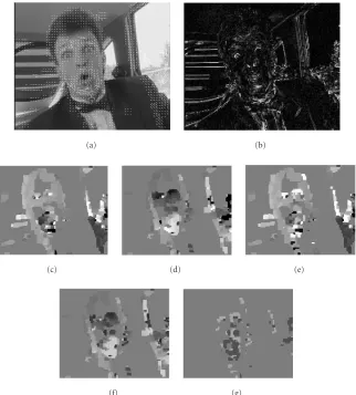
The first sequence examined isCarphone. The same frames (QCIF format), numbers 168 and 171, considered in [17] have been processed to make a possible comparison with some numerical results presented in that paper.

(6)

(a) (b)

(c) (d) (e)

(f) (g)

Figure3: Real world sequence (Carphone): (a) frame 171 with the superimposed motion field estimated through the proposed method;

(b) pixel-per-pixel squared diﬀerence between frame 171 and its motion compensated version; estimates obtained by means of the proposed method: the displacements (c)dxand (d)d y, the motion parameters (e)e, (f)f, and (g)θ.

side of the image and near the chin of the man, contain some wrong nonhomogeneous vectors. In particular, the er-rors visible on the objects at the right extreme of the window are due to the fact that these objects were not present in the previous frame, thus confusing motion estimation. On the other side, the few not well-estimated vectors on the chin cor-respond to uniform grey-level regions of the face, where local motion estimation algorithms often encounter problems. In Figure 3ba pixel-per-pixel squared diﬀerence between frame 171 and its motion compensated version is depicted. A clear gray level means a high discrepancy between the two im-ages; also in this picture significant errors are confirmed in the same areas as before. To better evaluate the obtained re-sults, inTable 2the value of prediction error (PE), computed with the proposed method, is compared to the data provided in [17], regarding the same sequence, and to H&S technique [1]: the proposed method performs better with respect to the other kind of approaches. In Figures3cand3dthe com-puted displacements (dxanddy) are also depicted. Finally, in Figures3e,3f, and3gthe motion parameters, respectively,

Table2: PE for Carphone sequence (higher value means a better

prediction). The results for the first three methods are taken from [17].

Kind of adopted approach PE

Block-based prediction [17] 31.8 dB Pixel-based prediction [17] 35.9 dB Region-based prediction [17] 35.4 dB

Horn&Schunck 30.4 dB

Proposed method 36.7 dB

(7)

(a) (b)

(c) (d) (e)

(f) (g)

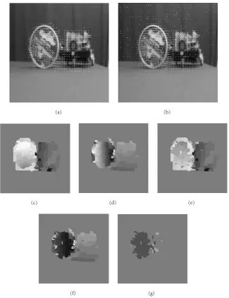
Figure4: Real world sequence (Robox): frame 15 with the superimposed motion field estimated through (a) the proposed method and (b)

the H&S approach; estimates by means of the proposed method: the displacements (c)dxand (d)d y, and the motion parameters (e)e, (f)

f, and (g)θ.

correspondence of the mouth and of the nose where motion is quite complex, and small rotational components are de-tected by the algorithm.

5.2.2. Robox

Experimental tests carried out with sequence namedRobox are illustrated inFigure 4and discussed in the sequel; frames taken into consideration are numbers 15 and 17. This se-quence is composed by two moving objects: a round box which rotates clockwise over a table and a small robot mov-ing towards the camera. In Figures4aand4b, frame 15 of the sequence with the motion field superimposed, computed, re-spectively, by means of the proposed method and through the H&S technique, is pictured. It can be easily noted how the motion field is more properly and precisely detected in

Figure 4awith respect to the other methodology, in particu-lar, for the rotating object.

(8)

(a) (b)

(c) (d) (e)

(f) (g)

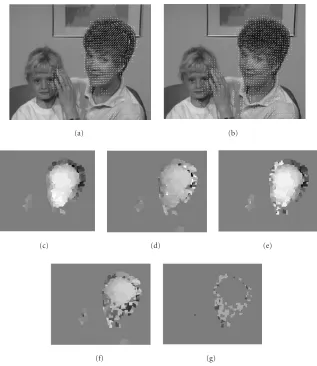
Figure5: Real world sequence (M&D): frame 39 with the superimposed motion field estimated through (a) the proposed method and (b)

the H&S approach; estimates by means of the proposed method: the displacements (c)dxand (d)d y, and the motion parameters (e)e, (f)

f, and (g)θ.

(Figure 4c) and has got values in displacementd yincreasing in magnitude going from its center towards the top and the bottom, thus resulting in correct description of a zooming eﬀect. In Figure 4gthe parameterθ is illustrated; only co-eﬃcients related to pure rotation (the box) are detected. As done before, also in this case, the PE has been computed and its value is reported inTable 3.

5.2.3. Mother&Daughter

Experimental tests carried out with a sequence called Mother&Daughter are presented in Figure 5 and debated hereafter.

In this video a mother caressing her daughter hair is de-picted; the mother moves her head towards right and, in ad-dition, slightly rotates up her neck; frames (QCIF format) that have been considered are numbers 38 and 40. In Fig-ures5aand5bthe motion vector field respectively estimated by the proposed methodology and the H&S approach are presented. It appears immediately that, in the first case, the field obtained is smoother and the vectors are very similar

(9)

Table3: PE for Robox sequence (higher value means a better pre-diction).

Table4: PE for sequenceM&D(higher value means a better

pre-diction).

in Figures5cand5d. In Figures5e,5f, and5gthe estimated motion parameters are presented. Figures 5e and 5f look quite similar to Figures5cand5dalready analyzed in detail. On the contrary, Figure 5gcontains very interesting infor-mation because it clearly indicates that there is an object with an anticlockwise rotation (bright gray pixels) and its rotation center can easily be supposed to be in the middle of the cir-cular region individuated. Also in this case the PE has been computed and its value is reported inTable 4.

6. CONCLUDING REMARKS

A new approach aiming at direct estimation of motion pa-rameters in a sequence of images has been developed. The method is based on the minimization of a potential function which is composed by two basic components accounting for frame matching and smoothness binding, respectively. This potential has been derived by exploiting MAP criterion and MRF modelling. The technique has given positive results both with synthetic and with real world sequences. In par-ticular, in addition to allow the direct estimation of motion parameters, the proposed technique shows excellent results also from the point of view of correct motion prediction (as demonstrated by the superior PE performances). This is due to fact that our approach constraint the estimated motion to adapt to a precise model, thus reducing the eﬀects of noise. The main drawback of the algorithm, as for most of MRF-based techniques, is the high computational cost. To improve this aspect, to enhance the precision of parameter estimate, and to better handle large displacements, a multiresolution approach is under investigation. Work is also in progress to adapt the algorithm to deal with a more complex kind of tion (zooming objects) by introducing a more general mo-tion model composed by a higher number of parameters.

REFERENCES

[1] B. K. P. Horn and B. G. Schunck, “Determining optical flow,” Artificial Intelligence, vol. 17, no. 1–3, pp. 185–203, 1981. [2] J. Konrad and C. Stiller, “On Gibbs-Markov models for

mo-tion computamo-tion,” in Video Compression for Multimedia Computing - Statistically Based and Biologically Inspired Tech-niques, H. Li, S. Sun, and H. Derin, Eds., pp. 121–154, Kluwer

Academic Publishers, Boston, Mass, USA, June 1997. [3] A. M. Tekalp, Digital Video Processing, Prentice-Hall,

Engle-wood Cliﬀs, NJ, USA, 1995.

[4] A. C. Bovik,Handbook of Image & Video Processing, Academic Press, New York, NY, USA, 2000.

[5] C. Stiller, “Object-based estimation of dense motion fields,” IEEE Trans. Image Processing, vol. 6, no. 2, pp. 234–250, 1997. [6] J. Konrad and E. Dubois, “Bayesian estimation of motion vec-tor fields,”IEEE Trans. on Pattern Analysis and Machine Intel-ligence, vol. 14, no. 9, pp. 910–927, 1992.

[7] E. C. Hildreth, “Computations underlying the measurement of visual motion,”Artificial Intelligence, vol. 23, no. 3, pp. 309– 354, 1984.

[8] H.-H. Nagel, “On the estimation of optical flow: Relations between diﬀerent approaches and some new results,”Artificial Intelligence, vol. 33, no. 3, pp. 299–324, 1987.

[9] L. Alparone, M. Barni, F. Bartolini, and R. Caldelli, “Regu-larization of optic flow estimates by means of weighted vector median filtering,”IEEE Trans. Image Processing, vol. 8, no. 10, pp. 1462–1467, 1999.

[10] J. Konrad and E. Dubois, “Estimation of image motion fields: Bayesian formulation and stochastic solution,” inProc. IEEE Int. Conf. Acoustics, Speech, Signal Processing, pp. 1072–1075, April 1988.

[11] L. Lucchese, “A frequency domain technique based on energy radial projections for robust estimation of global 2D aﬃne transformations,”Computer Vision and Image Understanding, vol. 81, no. 1, pp. 72–116, 2001.

[12] R. Y. Tsai and T. S. Huang, “Estimating three-dimensional motion parameters of a rigid planar patch,” IEEE Trans. Acoustics, Speech, and Signal Processing, vol. 29, no. 6, pp. 1147–1152, 1981.

[13] S. Geman and D. Geman, “Stochastic relaxation, Gibbs dis-tributions, and the Bayesian restoration of images,” IEEE Trans. on Pattern Analysis and Machine Intelligence, vol. 6, no. 6, pp. 721–741, 1984.

[14] J. Besag, “On the statistical analysis of dirty pictures,” J. Roy. Statist. Soc. Ser. B, vol. 48, no. 3, pp. 259–279, 1986.

[15] F. Heitz and P. Bouthemy, “Multimodal estimation of dis-continuous optical flow using Markov random fields,” IEEE Trans. on Pattern Analysis and Machine Intelligence, vol. 15, no. 12, pp. 1217–1232, 1993.

[16] M. M. Chang, M. I. Sezan, and A. M. Tekalp, “An algorithm for simultaneous motion estimation and scene segmentation,” inProc. IEEE Int. Conf. Acoustics, Speech, Signal Processing, vol. 5, pp. V/221–V/224, Adelaide, Australia, May 1994. [17] C. Stiller and J. Konrad, “Estimating motion in image

se-quences,” IEEE Signal Processing Magazine, vol. 16, no. 4, pp. 70–91, 1999.

Roberto Caldelliwas born in Figline Val-darno (Florence), Italy, in 1970. He grad-uated (cum laude) in electronic engineer-ing from the University of Florence, in 1997, where he also received his Ph.D. degree in computer science and telecommunications engineering in 2001. He works now as a Postdoctoral Researcher with the Depart-ment of Electronics and Telecommunica-tions at the University of Florence. He holds

(10)

Franco Bartoliniwas born in Rome, Italy, in 1965. In 1991, he graduated (cum laude) in electronic engineering from the Univer-sity of Florence, Florence, Italy. In Novem-ber 1996, he received his Ph.D. degree in informatics and telecommunications from the University of Florence. Since November 2001, he has been an Assistant Professor at the University of Florence. His research in-terests include digital image sequence

pro-cessing, still and moving image compression, nonlinear filtering techniques, image protection and authentication (watermarking), image processing applications for the cultural heritage field, signal compression by neural networks, and secure communication pro-tocols. He has published more than 130 papers on these topics in international journals and conferences. He holds three Italian and one European patents in the field of digital watermarking. He is a Member of the Program Committee of the SPIE/IST Workshop on Security, Steganography, and Watermarking of Multimedia Con-tents, and Technical Program Cochair of the IEEE MMSP Work-shop 2004. Dr. Bartolini is a Member of IEEE, SPIE, and IAPR.

Vittorio Romagnoliwas born in Abbadia S. Salvatore (Siena), Italy, in 1976. In 1994 he got the High School degree in industrial electronic from the “I.T.I.S. Amedeo Avo-gadro” in Abbadia S. Salvatore. In Febru-ary 2001 he graduated (cum laude) in elec-tronic engineering from the University of Florence with a thesis on motion estima-tion in video sequences. From March 2001 to September 2002, he worked in a