FULL PAPER
VHF radar measurements of momentum
flux using summer polar mesopause echoes
Iain M. Reid
1,2*, Rüdiger Rüster
3, Peter Czechowsky
3and Andrew J. Spargo
2Abstract
We revisit previously unpublished analysis of observations of the dynamics of the mesopause region over the Nor-wegian Island of Andøya (69°N, 16°E) made during a 1-week period in summer 1987 during the Middle Atmosphere Cooperation-Summer in Northern Europe (MAC-SINE) campaign using the mobile SOUSY VHF (53.5 MHz) Doppler radar operating in a six-beam mode. We do this in the light of: (1) more recent developments in the measurement of the components of the density-normalized Reynolds stress tensor using meteor radars, and with medium-frequency partial reflection radars using the hybrid Doppler interferometric technique, and (2) satellite measurements of the absolute upward flux of horizontal momentum. We consider of the density-normalized total upward flux of horizontal momentum u′w′+v′w′ for the 83–90 km height interval. Values of the component of the density-normalized flux for the 6 min to 12.8 h period range, after the tidal components have been removed, and the effects of the aspect sensitivity on the radar beam look directions have been accounted for vary between 5 m2 s−2 below 86 km and 13 m2 s−2 above 86 km. The major contribution is from the 6 to 12.8 h period range. The results of the analysis have implications for meteor radar estimates of momentum flux and also for Doppler radar measurements of the same term in the presence of aspect-sensitive scattering.
Keywords: Very high-frequency radar, Momentum flux, Polar mesosphere summer echoes
© The Author(s) 2018. This article is distributed under the terms of the Creative Commons Attribution 4.0 International License (http://creat iveco mmons .org/licen ses/by/4.0/), which permits unrestricted use, distribution, and reproduction in any medium, provided you give appropriate credit to the original author(s) and the source, provide a link to the Creative Commons license, and indicate if changes were made.
Introduction
The challenge of the measurement of the upward flux of horizontal momentum in the mesosphere lower thermo-sphere (MLT) region has been explored since the work of Vincent and Reid (1983), hereinafter VR83, which pre-sented a method for doing this using multi-beam Dop-pler radars, using only the assumption that the statistics of the wave field are horizontally isotropic. The meas-urement of this parameter is considered vital for better understanding the dynamics of the MLT (see, e.g. Fritts and Alexander 2003; Alexander et al. 2010). Progress has been made in using satellite measurements to estimate the absolute momentum flux of quasi-monochromatic gravity wave events (see, e.g. Hertzog et al. 2012; Ern et al. 2016). However, unlike these methods, the method applied by VR83 provides a measure of the net momen-tum flux and does not require identification of individual
gravity waves or assumptions beyond that of the statis-tical similarity of the wave field measured in the radar beams. This is important, as Reid et al. (1987) estimated that in a cross-spectral analysis of several radar data sets to determine gravity wave horizontal scales, only 25% of calculated cross-spectral phases had a significant coher-ence-squared [(COH)2] statistic. This can be interpreted
as quasi-monochromatic (QM) waves being evident only about 25% of the time, a rate consistent with the fre-quency of occurrence of QM waves in OI and OH air-glow observations (see, e.g. Reid and Woithe 2005).
Meek et al. (1985) also analysed almost a year of radar observations made near Saskatoon, Canada, for grav-ity wave horizontal scales and found a similar statistic. Walterscheid et al. (1999) analysed OH airglow imager data and found a higher frequency of occurrence of QM waves, varying from 41% of the observational time in winter, to 62% in summer. Reid et al. (1987), Reid and Woithe’s (2005) and Walterscheid et al.’s (1999) obser-vations are all for data from Adelaide, Australia. Based on these observational studies, we could argue that QM
Open Access
*Correspondence: ireid@atrad.com.au
1 ATRAD Pty Ltd, 20 Phillips St., Thebarton 5031, Australia
waves are present between 25 and 60% of the time. An additional complication in this context is whether the QM waves detected in airglow observations are freely propagating or ducted waves. The radar observations ref-erenced above were able to identify features consistent with propagating gravity waves over a range of heights, whereas single-colour airglow observations are single height measurements, and so restricted in interpretation. This is an important topic, but its further discussion is beyond the scope of the present work.
Naturally, the effects of instrumental filtering need to be considered when discussing the representativeness of observations, and VR83, Reid et al. (1987), Reid and Woithe (2005) and Meek et al. (1985) all explicitly do this for their observations of gravity wave scales. More generally, Gardner and Taylor (1998) consider the obser-vational limitations of gravity wave observations using lidar, radar and airglow observations. More recently, Bossert et al. (2018) have considered the measurement of momentum flux using a Na density lidar and included the chemistry of the Na response to the mountain waves. We note that the VR83 approach is not valid in the case of stationary waves. In terms of radar and Doppler lidar measurements of momentum flux, the approach of VR83 does not indicate a scale or temporal dependence in the governing equations, beyond the assumption that the statistics of the motions are horizontally homogeneous, and this was investigated by Reid (1984, 1987) using sim-ple analytical arguments. Perhaps the best way to further investigate this is through the use of simulations, and we consider some aspects of this approach below.
VR83 used the large medium-frequency (MF) Buck-land Park (BP) partial reflection (PR) radar [see Reid (2015) for a detailed discussion of this radar class], which provided good spatial and temporal coverage in the 60–95 km (day) and 80–95 km (night) height region. Powerful mesosphere–stratosphere–troposphere (MST) radars operating in the lower very high-frequency (VHF) band (typically near 50 MHz) can apply the technique but are limited by the temporal and spatial intermittency of the radar returns in the mesosphere lower thermosphere (MLT) region. Generally, in the MLT region outside of the polar mesosphere in summer, they are limited to day-time observations between 60 and 80 km. These radars are also relatively expensive and rare, and so alternate methods of measuring the momentum flux using smaller radars and optical techniques have been explored. These include an investigation of the ability of small interfero-metric MF PR radars to measure the flux by Thorsen et al. (1997), and an extension of Thorsen’s approach for application to ‘all-sky’ meteor radars (see, e.g. Holds-worth et al. 2004) by Hocking (2005). Except for recent work by Spargo et al. (2017), the former technique has
not been actively pursued. The approach described by Hocking has attracted much investigation, but no defini-tive experimental validation against an accepted meas-urement of momentum flux (see, e.g. Placke et al. 2015). For the various parts of the arguments for and against using the meteor technique for measuring momentum flux, see for example, the discussions in Vincent et al. (2010), Fritts et al. (2012), Riggin et al. (2016), and Spargo et al. (2017).
The strong radar returns from the summer polar mesopause region do provide a means of measuring the momentum flux in the MLT using more powerful VHF ST class radars (those with a power aperture product greater than around 107 W m2), at least in the 82–92 km
height region, with relatively good spatial and temporal coverage (see, e.g. Reid et al. 1988; Rüster and Reid 1990; Love and Murphy 2016). Given the relative sparsity of such measurements, the analysis and discussion of previ-ously unpublished momentum flux results is useful.
Observations
Observations were obtained as part of the international Middle Atmosphere Cooperation/Summer in Northern Europe (MAC/SINE) campaign (Thrane 1990) conducted in summer 1987 using the mobile SOUSY VHF Doppler Radar located at Bleik (69°17′N, 16°01′E) on the Norwe-gian Island of Andøya. The radar operated for a period of 32 days with various range resolutions, pulse codes and experiments, and useful mesospheric velocities were typically obtained within the height range of about 80 to 90 km. Other results from the MAC/SINE campaign using data from the same radar and relevant to the pre-sent work have been published by Reid et al. (1988), Rüster and Reid (1990), Rüster (1992), Lübken et al. (1990), and Yi (2001). The observational period for the results analysed in this paper is 22–30 June 1987. Previ-ously, Reid et al. (1989) looked at momentum flux meas-urements for the period of a few hours during 16–17 July and Rüster and Reid (1990) looked at measurements for the 23–25 June a period that covered that of the “Chaff” rocket salvo of the campaign (see, e.g. Wu et al. 2001). Equipment
of 576 four-element Yagi antennas, covering an effective area of 8880 m2, with a gain of 35.5 dB, and a one-way
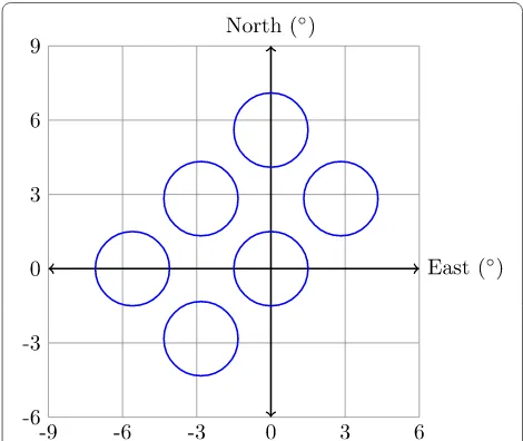
3 dB beam width of 3°. After Czechowsky et al.’s (1984) description of the radar, the number of beams was increased from four to six. In the configuration applied for the work described here, all six independent beams were utilized. Using electronically controlled phase shift-ers, the antenna beam was directed sequentially towards the six beam directions. Beams were directed vertically (V), and at 5.6° off-zenith towards the north (N) and west (W), and at 4.0° off-zenith towards the north-east (NE), north-west (NW) and south-west (SW). The beam con-figuration is illustrated schematically in Fig. 1. At a height of 86 km, the distance from the zenith to the centres of the 4.0° off-zenith beams is about 6 km, and for the 5.6° off-zenith beams, 8.4 km. The beam diameters are about 4 km at this height. The mobile SOUSY radar was relo-cated to Svalbard to become the SOUSY Svalbard Radar (SSR) in the late 1990s and is described by Czechowsky et al. (1998), and by Hall (2009).
Theory
Reynolds stress terms
The general case of the application of narrow beam Dop-pler radars to measure the density-normalized Reyn-olds stress tensor and mean winds in the MLT has been described by Reid (1987), and the theory for the beam arrangement used here has been described by Reid et al.
(1988). In the present case, apart from the mean square vertical velocity w′2 , the individual terms of the
Reyn-olds stress tensor are not available separately and come as combinations of terms. Briefly, the mean square radial velocities measured in the NE ( V′2
NE ) and SW ( V
′2
SW )
directed antennas can be used to determine the arith-metic sum of the upward fluxes of zonal ( u′w′ ) and
are the zonal, meridional and vertical perturbation velocities, respectively, the subscripts on the variances of the radial velocities indicate the beam directions, and θE1 is the effective beam direction for the
NE and SW beams. (We discuss the calculation of the effective beam direction below.) This expression may be compared with the mean absolute flux (MF) typically measured by satellite and balloon measurements (e.g. Hertzog et al. 2012) as
The isotropy of the horizontal velocity field can also be calculated directly from the mean square radial velocities measured in the N ( V′2
N ) and W ( V
′2
W ) beams as
where θE2 is the effective beam direction for the N and W
beams. The isotropy is one of the Stokes parameters, and Eckermann (1996) provides a detailed description of the use of these parameters in the analysis of wave fields. We note that spectral rotary decomposition and the applica-tion of the Stokes parameters is usually most useful for longer (inertial) wave periods.
The mean square horizontal velocities cannot be obtained separately without further information, as they are given by (using the meridional component as an example)
and where a similar expression applies for the zonal com-ponent. Note that this is the expression that applies for the usual beam arrangement (a vertical beam and an off-vertical beam in the east–west and north–south plane) for most Doppler radars, and Eq. (4) is usually applied
(1)
to calculate the mean square horizontal velocity. Also note that the inability to separate the individual terms in our experiment comes about because the beam point-ing angles all lie in one half-azimuth. A similar situation occurs with the azimuthal distribution of meteor radar detections as the Earth rotates into the meteor streams during the day. We will return to the importance of this below.
Another point to note when considering Eqs. (1), (3) and (4) is that they apply equally to the mean square spectral widths, σ′2 and so can be used to investigate
scales smaller than the radar pulse volume (Reid 2004), although this appears to have been little exploited.
Rather than using individual combinations of beams as we have just described, it is possible to include all of the radial velocities in a least-squares inversion to determine the mean wind components and the various covariance terms of the Reynolds stress tensor. Spargo et al. (2017) did this, following the approaches of Thorsen et al. (1997) and Hocking (2005), to determine the six components of the density-normalized Reynolds stress tensor, to the BPMF radar operating in a five-beam (E, W, N, S and V) Doppler mode. In principle, this technique can be applied to the six-beam arrangement used here to deter-mine the various Reynolds stress terms. This is in some ways a test of the attempts to measure them from meteor radar radial velocity data, particularly given the asym-metrical distribution of meteor returns around the zenith throughout the day.
The inversion is performed on the following system of equations (constituting n radial velocity measurements):
where VR′2 represents an n-element vector of squared
We applied the least-squares inversion to calculate the individual variances and covariances corresponding to the Reynolds stress tensor terms from our data (follow-ing the removal of tidal and longer period components as described below) and found the results to be physically unreasonable except for w′2 , and extremely sensitive to
outliers in the radial velocity vector. This is not unex-pected given the governing equations described above and given that we have a direct measure of w′2 . In
addi-tion, the sensitivity to changes in the radial velocity vec-tor is expected to arise and occurs when solving inverse problems where the so-called coefficient matrix (here containing the direction cosines) has a high condition
(5)
V′2 R =Av
number [see, e.g. Shenghui et al. (2014)]. In our case, the high condition number is predominantly brought about by the small direction cosines associated with those covariance terms which involve a horizontal component. The condition number of our problem is also further increased by the fact that the beam locations have little spatial separation, as we have allowed them to vary solely as a function of the estimated aspect sensitivity.
Our interpretation is that in solving the inverse prob-lem for this beam geometry, large correlated errors will predominantly accumulate in those components that include horizontal terms. As a consequence, we have lit-tle confidence in the solutions the inversion algorithm produces for individual components involving a horizon-tal term (i.e. u′u′ , v′v′ , u′v′ , u′w′ and v′w′ ). This warrants
further discussion though, and the governing equa-tions do not preclude the soluequa-tions for
u′w′+v′w′ and
(v′2−u′2) , and when applied for these terms, the
inver-sion yields similar results to the application of Eqs. (1) and (3) and confers advantages in terms of robustness and correcting for the effects of aspect sensitivity. We will return to this in the “Momentum flux” section, and in the “Simulation” section, where we show results from a simu-lation comparing the measurement biases inherent to the least-squares inversion and radial velocity variance differ-encing techniques.
Effective beam direction
The need to calculate an effective Doppler beam direc-tion comes about because of the high aspect sensitivity of backscatter often returned from the atmosphere along with the relatively wide Doppler beams used with atmos-pheric radars (see, e.g. Reid 1990). The most commonly applied approach to account for this for fixed beam Dop-pler radars is described by Hocking et al. (1986), but also see similar work by Whitehead et al. (1983). Its applica-tion to the mobile SOUSY and Harz SOUSY radar data has previously been described by Reid et al. (1988), Czechowsky et al. (1988) and Reid et al. (1989). Its appli-cation to a subsection of the present data set has been described by Rüster and Reid (1990). Briefly, the ratio of powers measured in a vertical beam, P(0) , and a beam
directed at an apparent off-vertical angle, θA , P(θA) , can be used to determine the effective beam angle as
where θ0 is the is the 1/e radar beam half-width, and θs
The spectral half-width due to beam broadening, f1/2 ,
can also be calculated using the values of θs as (Hocking
et al. 1986)
Reid (2004) argued that beam broadening and shear broadening effects could be ignored when the beams were symmetric, for example, with beams at the same off-zenith angle in either the east–west or north–south plane, because they would be affected in the same way, and the terms due to these effects would subtract out. If this argument is correct, then Eq. (1) can be applied to spectral widths without using the correction indicated by Eq. (8).
Analysis
SNR, radial velocities and spectra widths
Radar returns were coherently integrated for 0.107 s, and for each beam position 64 such complex samples were obtained in each of the 135 range intervals. Data were thus obtained for 6.8-s in each of the beam directions. A new data sequence was started every 10 s, the addi-tional time being required to switch the beam direction, and to write data to tape. The 6.8-s data sequences were Fourier transformed off-line to obtain the corresponding Doppler spectra. The first three moments of the spec-tra were calculated to obtain the power, mean Doppler shift and spectral width. Spectra were required to have signal-to-noise ratios exceeding 3 dB to be accepted and were checked for aliasing. The latter occurred when radial velocities exceeded 13.1 ms−1 and were removed
by accounting for the spatial and temporal variation of the signals at each range gate and beam position. These results were averaged to produce 3-min records in each height step, and in each beam.
The mean power profiles for the six beams and the acceptance rates for the 3-min records are shown in Fig. 2. The acceptance rates follow the form of the power profiles and take maximum values of about 70% for the vertical and northward beams, and values of 40% near ranges of 83 and 90 km, respectively. The westward beam has the lowest powers and acceptance rates of all of the beams. When we consider the momentum flux, and its divergence with height, the strong height dependence of these rates must be kept in mind. The limited height
(7)
range over which radial velocities are available for analy-sis highlights the limitations of using this class of radar to measure the fluxes. Meteor radars are similarly limited, with a similar form for the acceptance rate with height, suggesting some inherent advantages in using MF partial reflections radars, although these bring their own limi-tations (see Reid 2015). We discuss the θs and θE results
below.
The signal-to-noise ratios (SNRs), radial velocities and spectral widths for the 3-min averaged data are typical for this type of observation in that they are character-ized by substantial temporal and spatial variability. There are periodic ‘gaps’ in the returns, and the SNRs show the influence of the semidiurnal tide in the modulation of the strength of the returned signals. This has previously been discussed by Czechowsky et al. (1989) in relation to the PMSE, who noted that strong bursts in backscattered power tended to occur in the late afternoon and early morning hours, coinciding with the time of maximum westward velocity of the semidiurnal tide. Czechowsky and Rüster (1997) noted and discussed the tendency for the spectral width to maximize above about 86 km, and this is evident in the present data set. They con-cluded that this was the result of the presence of cells of enhanced turbulence generated by a Kelvin–Helmholtz (KH) mechanism. This would lead to reduced aspect sen-sitivity in the upper parts of the PMSE, consistent with the results shown in Fig. 2. We note that clear signatures of KH instabilities were observed in wintertime using this radar by Reid et al. (1987), and more recently in PMSE over Andøya by Stober et al. (2018).
Mean scattering angle and beam pointing angles
The mean power profiles can be used to calculate the mean scattering angle θs and the mean effective angle θE
for each of the beams for the entire period of observation, and these results are also shown in Fig. 2. To calculate θs
and θE the power profiles for the off-zenith beams were
interpolated back to their nominal height (that is, assum-ing θE=θA ). If θs could not be calculated using Eq. (6), θE was set to θA . These mean scattering angle results are similar to others found in the PMSE using the same tech-nique (see, e.g. Reid 1990), but we note the considerable variability of θs calculated from the different off-zenith
beams, and that θs is higher at the base of the layer. If
discussed in more detail in Murphy and Vincent (1993) and Reid (2015). It has significant implications in apply-ing Eq. (1), as it assumes that a single value of θE is
avail-able and can be applied.
A mean over the entire week-long data set may not produce the most representative value of beam direc-tion on shorter time scales, and to highlight this, Fig. 3
shows the 21-min values of θs for the westward beam. A
clear statement on the variation with time and height is not evident, except that there is considerable variability. There is perhaps a tendency for θs to be larger nearer the
top of the layer. Figure 4 shows the mean effective angle corresponding to Fig. 3. While there is considerable vari-ability, the effective beam direction is often the apparent beam angle. This is a consequence of the narrow beams and relatively small off-zenith angles used for the non-vertical beams with this radar.
To further investigate the nature of the scattering angle, Fig. 5 shows examples of its distribution for three heights: 83.1 km (yellow); 85.8 km (red); and 88.8 km (blue) for the entire observational period for 21-min averages of power. The median values are 6.8°, 7.4° and
8.7°, respectively. These results represent the mean of 21-min averages. The number of values determined for each of these heights is 197, 348, 302 from a possible 502 (39%, 69% and 60%, respectively). For the remainder of the 21-min averages during the observational period, no value of θs could be determined. These results are similar
in form to those reported for a 51.5-MHz radar at Res-olute Bay (75°N, 95°W) for 1 month of hourly averaged observations by Swarnalingam et al. (2011).
This highlights some issues around the application of Eq. (6). It is best suited to small values of θs and becomes
increasingly insensitive as it increases. There is also a question around the most suitable time interval over which to calculate it. Reid et al. (1988) used a mean value calculated over a period of a few hours, and Rüster and Reid (1990) used a mean calculated over a period of 2 days, matching the periods over which they calculated momentum flux. To obtain a statistically valid measure of momentum flux, long averaging intervals of the mean square radial velocities are required (see, e.g. Vincent et al. 2010). During this period θs and hence θE will vary,
but the application of Eq. (1) requires a single value of
Fig. 2 Mean SNR for each of the beams for the entire observational period (top left), the radial velocity acceptance rates for each range for the six beams using a 3-dB acceptance criterion (top right), the scattering angle θs calculated from each of the off-zenith beams and the mean of these (in
θE for the averaging interval, so we have two competing
requirements. This problem is avoided by applying the least-squares inversion approach because it allows for a fit to the known radial velocities, each of which is associ-ated with an effective beam angle. This does require some care (e.g. Andrioli et al. 2013) and is not as simple mathe-matically as the application of Eq. (1), but in the presence of aspect sensitivity and relative wide Doppler beams, it may be the preferred approach.
Another question arises whether the off-zenith power exceeds that in the vertical direction, and whether this
means that there is a patchy layer present, a tilted layer present, or that the scattering is quasi-isotropic? If we accept the Gaussian fall-off in power used to derive Eqs. (6) and (7), then an off-vertical power in excess of the vertical power should be treated as indicating iso-tropic scatter. The effective beam direction should then be set to the apparent beam direction. Whatever the underlying mechanism, the need to correct for the effec-tive beam direction on some occasions remains. In the present work, the effect is not severe because the beam-widths are quite small, as are the off-zenith angles. With
Fig. 3 Scattering angle calculated from 21-min records for the westward beam
wider beam Doppler radars, this effect could be quite large.
In this work, we have calculated θs and hence θE for each 3-minute record for each beam where possible and substituted the apparent beam direction when not. We then averaged the θE values to obtain one value for each off-zenith angle, and used these in Eqs. (1), (3) and (4). We averaged the values of θE obtained from beams with the same off-zenith angles θA to obtain one θE1 and one θE2 for use in Eqs. (1) and (3). We also calculated the
mean value of θE1 and θE2 for the entire observing period
(Fig. 2) and used this in the same equations. We would expect the correct values of the Reynolds Stress terms to lie between these two values. We also applied the least-squares inversion approach, which fits to the radial velocities and their effective beam directions. We there-fore have three estimates for the Reynolds stress terms described by Eqs. (1), (3) and (4).
Alternate approaches to measuring θs using a
multi-receiver radars have been described by Murphy and Vincent (1993), Holdsworth and Reid (2004) and more recently by Sommer et al. (2016). Murphy and Vincent
(1993) and Holdsworth and Reid (2004) used multi-receiver techniques to look at mid-latitude MF partial reflections and is so not entirely applicable here. Sommer et al. also used a multi-receiver approach, but looked at the PMSE at VHF over Andøya, and so is directly relevant to the present work. They used both Eq. (6) and multi-receiver approaches and found larger values of θs than
other studies and so argued that their results generally indicated isotropic scattering, with periods of localized anisotropic scattering process leading to higher aspect sensitivity. This interpretation is not inconsistent with our results when we note that 61, 31 and 40% of records indicate isotropic scatter (or a failure to calculate θs at
least) at heights of 83.1, 85.8 and 88.8 km, respectively.
Mean winds and tides
The tidal components during this observational period have previously been discussed by Lübken et al. (1990), Manson et al. (1992) and Rüster (1992, 1994) for the entire MAC/SINE campaign, and further details on the results of the analysis of the mean and tidal winds may be found therein. However, these components need to
be removed from the radial velocity time series, and so we describe the approach used to calculate and remove them and note a few details. To calculate the mean and tidal winds, we follow the approach used by Spargo et al. (2017) for the BPMF Doppler radar (Reid et al. 1995; Holdsworth and Reid 2004) operating in Hybrid Dop-pler Interferometer (HDI) mode, and which is similar to that applied by Andrioli et al. (2013) to meteor radar radial velocities. Briefly, the radial velocities were parti-tioned into non-oversampled windows of width 1 h, and the three wind components (u,v,w) were estimated using
a standard least-squares formulation (e.g. Vandepeer and Reid 1995). The major periods present were deter-mined using a Lomb periodogram, and these periods were removed from each radial velocity by subtracting from them a time-dependent radial projection of a least-squares fit y to the wind time series, of the form:
where T is an n-element array of the significant periods,
and Φ is an n-element array of phases providing the time
at which the ith component maximizes. The fits were made over windows of length 48 h. These time series were then used in any further analysis requiring the radial velocities. This is more computationally invasive approach than that of VR83.
(9)
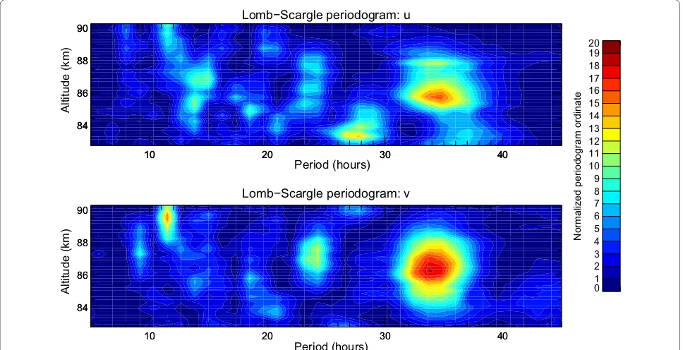
Figure 6 shows the Lomb periodogram for the zonal and meridional wind components. Inspection of this fig-ure indicates pronounced periodicities at 8, 12 and 24 h, and also near 28, 32 and 36 h. Rüster (1994) has discussed the nonlinear interaction of the various wind compo-nents during periods overlapping that of this data set and identified waves in the 32–38-h period range result-ing from nonlinear wave–wave interactions of the third order. In addition, he found the most frequently observed periods present were those corresponding to interactions between the dominating diurnal and semidiurnal tides and planetary waves with periods of 2–3 days. In addi-tion to second-order processes, higher-order interacaddi-tions were also observed in the velocity fluctuations and in the echo power, suggesting corresponding temperature vari-ations. We have removed the 8, 12 and 24 h tidal compo-nents, as well as the 18, 32 and 36 h periodicities evident in the Lomb periodograms using Eq. (9). The harmonic fitting limits the height coverage of the data, as it fails with limited data, and useable data are limited to heights between 82 and 91.6 km.
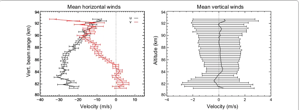
Figure 7 shows the mean zonal, meridional and vertical winds with the tidal components removed for the entire period of observation. The zonal wind field has a west-ward flow with a peak magnitude of about 30 ms−1. The
meridional wind is equatorward above 85 km and around zero below. The mean vertical wind is downwards below
10 20 30 40
84 km and upwards above, but given the uncertainties, is effectively zero.
Momentum flux
For the application of the VR83 approach, after removal of the tidal and other periodicities, the 3-min time series of radial velocities and spectral widths were filtered for periods less than 1 h, for periods between 1 and 6 h, and for 6 h to the inertial period (12.8 h). We only show the results for 6 min to 12.8 h here. To filter the time series, a spline was applied, and the splined values used to fill in missing data points. A fifth-order Butterworth filter with appropriate cut-offs was then applied to this modi-fied time series. Variances were then calculated for the filtered time series, using only values corresponding to those times when real data were obtained. All the time series were treated in the same way. Equations (1), (3) and (4) are then applied to the filtered time series. The effective beam directions were calculated using the pow-ers measured in each of the off-zenith beams relative to that measured in the vertical beam as described above. The momentum fluxes derived for scales larger than the radar pulse volume calculated using radial velocities we call ‘superscale’, and for scales smaller than the pulse vol-ume calculated using spectral widths, we call ‘subscale’. We calculate the superscale flux using both the VR83 and least-squares inversion approaches. We begin with the subscale results shown in Fig. 8.
Subscale momentum flux
For the subscales, momentum flux values for periods less than 12.8 h are generally between ±1.0 m2s−2 except at the lowest two heights where they are +2−3 m2s−2 ,
and we conclude that the momentum flux for subscales
for periods less than 12.8 h is essentially zero. We have not attempted to calculate the subscale momentum flux using the inversion technique. This result is in contrast to that of Reid (2004) who did find significant fluxes. In his case, the radar pulse volume was very much larger, approximately 4 × 13.5 km at 86 km altitude, compared
to 0.3 × 8 km here. To obtain the total arithmetic sum of
the momentum flux (u′ w′
+v′
w′) for all scales for periods
between 6 min and 12.8 h, the superscale and subscale momentum fluxes should be added. The small values of the subscale results mean that the total flux is essentially the same as that for the superscale flux in this case, which we now consider.
Superscale momentum flux
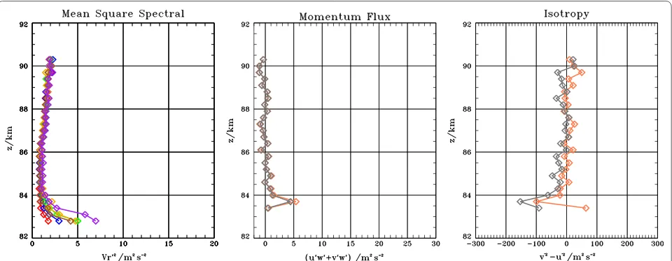
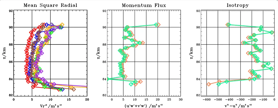
Figure 9 summarizes the mean square radial velocities, the arithmetic sum of the momentum fluxes (u′w′+v′w′)
and (v′2−u′2) for scales larger than the pulse volume for
periods less than 12.8 h, the inertial period. We note that the mean square radial velocities do show some noise, which propagates into the momentum flux and isotropy results. In this plot, we have shown the flux calculated using the apparent beam direction in green, and the flux calculated using the mean effective beam direction calcu-lated for all of the 3 min observations in coral. Inspec-tion of this plot indicates a 10–15% difference. Corrected flux values in coral are about 5 m2s−2 below 86 km,
and increase rapidly between 86.5 and 87 km to around
13 m2s−2 , before settling back to around 7.5 m2 s−2 above
about 88.5 km. The form of these plots suggests that more at the top, and less so at the bottom of the height range, values may not be representative of the average for the whole observational period. Figure 10 shows the results from the inversion approach. The form is very
−40 −30 −20 −10 0 10
similar to that of Fig. 9, and the values similar. The error bars indicate the one sigma standard deviations. The pro-file is perhaps less noisy than that for the VR83 approach, but clearly, the same values are being measured. For both approaches, the isotropy is negative, with values of between − 50 m2 s−2 at the lowest heights, and about − 200 m2 s−2 above.
Simulations
We noted in “Reynolds stress terms” section that the general inversion of the radial velocities to determine the individual terms of the Reynolds stress tensor failed to deliver physically realistic results. To provide further insight into this, we simulated the present beam arrange-ment in the presence of a gravity wave field following the approach of Spargo et al. (2017).
Briefly, the simulation incorporated a superposi-tion of 37 gravity waves with periods in the range of 10–180 min, with randomly selected initial phases and propagation directions in the Eastern sector. This dis-tribution of wave directions led to negative values of
u′w′ , and near-zero values of v′w′ . Diurnal and
semi-diurnal tides were also included in the wave field and were removed using the same approach as discussed in the “Mean winds and tides” section. Each covari-ance estimation was performed over a 48-h segment of simulated data. A total of 10000 realisations were per-formed, so as to be able to qualitatively illustrate the bias distribution. To simulate realistic changes in beam position, we assumed an aspect sensitivity in the model randomly varying between 5° and 15° in a temporally
correlated random manner, with a spectrum corre-sponding to that of the power-law temporal spectrum model in Eq. (24) of Gardner et al. (1993). Gaussian dis-tributed errors were added to the “measured” zonal and meridional zenith angles of the beam positions, with standard deviations of 0.25°.
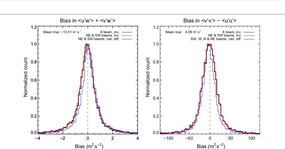
The results are shown in Fig. 11. Agreement between the VR83 approach and the least-squares inversion for both two and six beams is very good for the determina-tion of the arithmetic sum of the fluxes. The isotropies are also in excellent agreement. We note that attempt-ing to solve for the individual flux terms led to non-physical values. As we noted above, we interpret this as an indication that large, correlated errors had accumu-lated in the u′w′ and v′w′ components.
In summary, based on simple modelling, the inversion technique appears to be equivalent to the VR83 tech-nique used for the analysis in this paper to determine the arithmetic sum horizontal momentum flux. We propose to further investigate ways to reduce the inverse prob-lem’s condition number, and its sensitivity to outliers. We note in this context that to deal with fitting radial veloci-ties to multisite FPI observations, Harding et al. (2015) successfully regularized the inversion problem in such a way as to produce “smooth” variations in the solved com-ponents. It is not clear how well the approach will lend itself to non-ideal observing geometries in the covariance estimation situation, but it nonetheless appears prom-ising, in particular for application to meteor radar esti-mates of wind covariance.
Summary and conclusion
For the total momentum flux for superscales and periods between 6 min and 12.8 h, values are typically between 5 and 13 m2 s−2. The contribution from the 6 to 12.8 h
period range dominates the other period bands. These results are consistent with those of Placke et al. (2015) who used the Saura MF radar, located close to the for-mer position of the mobile SOUSY radar, and the VR83 approach, to measure momentum flux and who provide the mean for June 2011. Their values for u′w′ and v′w′ are
both positive over the height region of our observations and take values of around 3 m2s−2 , so they are generally
consistent but smaller than our results when applying the same technique. They also measured the fluxes using a nearby meteor radar. The results agree somewhat over a restricted range in summer. However, these authors did not correct for aspect sensitivity, nor did they remove the tidal components from their data, so there is some uncer-tainty around their results.
For the subscales, values are between ±1.0 m2s−2 and essentially zero. Simulations show that the estimates of the individual wind covariance terms from a least-squares inversion are erroneously correlated, but that the arithmetic sum of the horizontal fluxes, a term allowed by the beam geometry, is in excellent agreement with the VR83 technique (which is typically used to estimate momentum fluxes from this type of radar). We propose to further investigate ways to reduce the instability in the least-squares inversion approach.
Our results suggest that the validity of the least-squares inversion for meteor radar radial velocities to determine
momentum fluxes will depend on the azimuthal sym-metry of the meteor distribution. We have seen that with our beam arrangement, which is similar to a typical meteor distribution for a particular time of day, the Reyn-olds stress terms cannot be individually retrieved. Fur-thermore, unlike the arrangement in the present work, the meteor distribution rotates throughout the day. For meteor radars with relatively low counts where the asym-metry is typically significant, it would not be clear which combinations of terms are correct at particular times of the day, and the average over the day would be suspect. Simulation results presented by Spargo et al. (2017), do show acceptable recovery of the Reynolds stress terms when using actual meteor locations derived from the Buckland Park meteor radar, but actual experimental ver-ification of meteor radar measurements of momentum flux is still incomplete.
Inspection of the height coverage plot for the present results clearly indicates the limited height range over which representative results can be calculated (50% at 84 and 90 km, albeit at a very good range resolution of 300 m). This was a powerful radar, with an antenna area of 8880 m2, a peak power (for this work) of 100 kW, and
a duty cycle of 4% (3.55 × 10⁷ W m2). Together with the
ongoing uncertainty around the measurement of the Reynolds Stress tensor using meteor radars, this suggests that Doppler capable MF/HF partial reflection radars (e.g. Saura MF, Juliusruh MF and the Buckland Park MF), might be the reference instruments for this meas-urement, with height coverage from 60 to 94 km with 1–2 km height resolution. The limited height resolution
−10 −5 0 5 10 15 20 80
82 84 86 88 90 92
94 u’w’ + v’w’
−10 −5 0 5 10 15 20 80
82 84 86 88 90 92 94
Vertical beam height (km)
v’v’ − u’u’
−600 −400 −200 0 200 Covariance (m2 s−2)
Covariance (m2 s−2)
80 82 84 86 88 90 92 94
Vertical beam height (km)
Fig. 10 Superscale momentum flux obtained using the least-squares inversion approach. Values are very similar to those shown in Fig. 9, but are somewhat less noisy
−4 −2 0 2 4
0.0 0.2 0.4 0.6 0.8 1.0
1.2 Bias in <u’w’> + <v’w’>
−4 −2 0 2 4
0.0 0.2 0.4 0.6 0.8 1.0 1.2
Normalized coun
t
Mean true: −13.51 m2.s−2 6 beam, inv. NE & SW beams, inv. NE & SW beams, rvel. diff.
Bias in <v’v’> − <u’u’>
−100 −50 0 50 100 Bias (m2.s−2)
Bias (m2.s−2)
0.0 0.2 0.4 0.6 0.8 1.0 1.2
Normalized coun
t
Mean true: 4.09 m2.s−2 6 beam, inv. NE & SW beams, inv. SW, W, N & NE beams, rvel. diff.
Fig. 11 Bias in measurements of the arithmetic sum of the density-normalized momentum flux and isotropy using the VR83 technique (blue), and a two (red) and six (black) beam least-squares inversion calculated using a simulated gravity wave field. The left-hand panel shows the values of
u′w′+v′w′ for both the inversion-estimated case and that from the covariance calculated from the model’s Cartesian winds at a fixed point (i.e. an
may actually be an advantage, producing a natural ana-logue summing of the data into 2 km bins. A reduced height resolution, perhaps 600 m, on the MST may have also been an advantage.
We recommend the use of the inversion technique for multi-beam Doppler radars in the presence of aspect-sensitive scatter because of its variable nature, and the relatively broad beams of most real-world radars. In the application of the VR83 technique, Doppler Na lidars may have a real practical advantage in good seeing con-ditions because of their narrow beam widths, and strong returns from the 80 to 100 km height region.
Abbreviations
AOA: angle of arrival; BP: Buckland Park; (COH)2: coherence squared statistic; E,
W, N, S, V: east, west, north, south, vertical; HDI: hybrid Doppler interferometry; HF: high frequency; KH: Kelvin–Helmholtz; KHI: Kelvin–Helmholtz Instability; MAC-SINE: Middle Atmosphere Cooperation-Summer in Northern Europe; MF: medium frequency; MLT: mesosphere lower thermosphere; MST: mesosphere stratosphere troposphere; NE, NW, SW: north-east, north-west, south-west; PMSE: polar mesosphere summer echoes; PR: partial reflection; PRF: pulse repetition frequency; RADAR: radio detection and ranging; SOUSY: sounding system; SSR: SOUSY Svalbard radar; ST: stratosphere troposphere; VHF: very high frequency.
Authors’ contributions
IMR wrote this paper. RR did the original data reduction and produced the radial velocity, power and spectral width time series data further analysed here. PC implemented the six-beam antenna arrangement used for this study and provided overall management of the SOUSY involvement in MAC/SINE. AJS developed the gravity wave simulations and contributed to writing this paper. All authors read and approved the final manuscript.
Author details
1 ATRAD Pty Ltd, 20 Phillips St., Thebarton 5031, Australia. 2 School of
Physi-cal Sciences, University of Adelaide, Adelaide 5000, Australia. 3 Max Planck
Institute for Solar System Research, 37077 Göttingen, Germany.
Acknowledgements
The authors thank the staff of the Andøya Rocket Range and the members of the SOUSY project group of the Max-Planck-Institut für Aeronomie in obtain-ing the measurements.
Competing interests
The authors declare that they have no competing interests.
Availability of data and materials
Data requests should be made to IMR or to the Max Planck Institute for Solar System Research.
Funding
The antenna system of the mobile SOUSY VHF Radar was funded by the Deutsche Forschungsgemeinschaft. The original data analysis was partly carried out using the facilities of the Gesellschaft für wissenschaftliche Datenverarbeitung in Göttingen. The involvement of IMR in the preparation of this paper was supported by ATRAD Pty Ltd. AJS is supported by an Australian Commonwealth postgraduate scholarship.
Publisher’s Note
Springer Nature remains neutral with regard to jurisdictional claims in pub-lished maps and institutional affiliations.
Received: 27 February 2018 Accepted: 2 August 2018
References
Alexander MJ, Geller M, McLandress C, Polavarapu S, Preusse P, Sassi F, Sato K, Eckermann S, Ern M, Hertzog A, Kawatani Y, Pulido M, Shaw TA, Sigmond M, Vincent R, Watanabe S (2010) Recent developments in gravity-wave effects in climate models and the global distribution of gravity-wave momentum flux from observations and models. Q J R Meteorol Soc 136:1103–1124. https ://doi.org/10.1002/qj.637
Andrioli VF, Fritts DC, Batista PP, Clemesha BR (2013) Improved analysis of all-sky meteor radar measurements of gravity wave variances and momentum fluxes. Ann Geophys 31:889–908. https ://doi.org/10.5194/ angeo -31-889-2013
Bossert K, Fritts DC, Heale CJ, Eckermann SD, Snively JB, Williams BP, Reid IM, Murphy DJ, Spargo AJ, MacKinnon AD (2018) Spectral momentum flux of a mountain wave event over New Zealand. J Geophys Res Atmos. https :// doi.org/10.1029/2018J D0283 19
Czechowsky P, Rüster R (1997) VHF radar observations of turbulent structures in the polar mesopause region. Ann Geophys 15:1028–1036. https ://doi. org/10.1007/s0058 5-997-1028-8
Czechowsky P, Schmidt G, Rüster R (1984) The mobile SOUSY Doppler radar: technical design and first results. Radio Sci 19(1):441–450. https ://doi. org/10.1029/RS019 i001p 00441
Czechowsky P, Reid IM, Rüster R (1988) VHF radar measurements of the aspect sensitivity of the summer polar mesopause echoes over Andenes (69°N,16°E), Norway. Geophys Res Lett 15:1259–1262. https ://doi. org/10.1029/GL015 i011p 01259
Czechowsky P, Reid IM, Rüster R, Schmidt G (1989) VHF radar echoes observed in the summer and winter polar mesosphere over Andøya, Norway. J Geophys Res 94(D4):5199–5217. https ://doi.org/10.1029/JD094 iD04p 05199
Czechowsky P, Klostermeyer J, Röttger J, Rüster R, Schmidt G (1998) The SOUSY-Svalbard-Radar for middle and lower atmosphere research in polar regions. In: Edwards B (ed) Solar-terrestrial energy program, Proceedings of 8th Workshop on Technical and Scientific Aspects of MST Radar, Bangalore/Indien 1997. SCOSTEP Secret., Boulder, pp 318–321.http://hdl.handl e.net/11858 /00-001M-0000-0014-DAC1-6 Eckermann SD (1996) Hodographic analysis of gravity waves: relationships
among Stokes parameters, rotary spectra and cross-spectral methods. J Geophys Res 101(D14):19169–19174. https ://doi.org/10.1029/96JD0 1578 Ern M, Trinh QT, Kaufmann M, Krisch I, Preusse P, Ungermann J, Zhu Y, Gille JC, Mlynczak MG, Russell JM III, Schwartz MJ, Riese M (2016) Satellite observa-tions of middle atmosphere gravity wave absolute momentum flux and of its vertical gradient during recent stratospheric warmings. Atmos Chem Phys 16:9983–10019. https ://doi.org/10.5194/acp-16-9983-2016 Fritts DC, Alexander MJ (2003) Gravity wave dynamics and effects in the
mid-dle atmosphere. Rev Geophys 41:1003. https ://doi.org/10.1029/2001R G0001 06
Fritts DC, Janches D, Hocking WK, Mitchell NJ, Taylor MJ (2012) Assessment of gravity wave momentum flux measurement capabilities by meteor radars having different transmitter power and antenna configurations. J Geophys Res 117:D10108. https ://doi.org/10.1029/2011J D0171 74 Gardner CS, Taylor MJ (1998) Observational limits for lidar, radar, and airglow
imager measurements of gravity wave parameters. J Geophys Res 103(D6):6427–6437. https ://doi.org/10.1029/97JD0 3378
Gardner CS, Hostetler CA, Franke SJ (1993) Gravity wave models for the hori-zontal wave number spectra of atmospheric velocity and density fluctua-tions. J Geophys Res 98(D1):1035–1049. https ://doi.org/10.1029/92JD0 2051
Hall CM, Röttger J, Kuyeng K, Sigernes F, Claes S, Chau J (2009) First results of the refurbished SOUSY radar: tropopause altitude climatology at 78°N, 16°E, 2008. Radio Sci 44:RS5008. https ://doi.org/10.1029/2009R S0041 44 Harding BJ, Makela JJ, Meriwether JW (2015) Estimation of mesoscale
ther-mospheric wind structure using a network of interferometers. J Geophys Res Space Phys 120:3928–3940. https ://doi.org/10.1002/2015J A0210 25 Hertzog A, Alexander MJ, Plougonven R (2012) On the intermittency of gravity
wave momentum flux in the stratosphere. J Atmos Sci 69(11):3433–3448. https ://doi.org/10.1175/JAS-D-12-09.1
Hocking WK (2005) A new approach to momentum flux determinations using SKiYMET meteor radars. ANGEO 23(7):2433–2439. https ://doi. org/10.5194/angeo -23-2433-2005
radar. J Atmos Terr Phys 48:131–144. https ://doi.org/10.1016/0021-9169(86)90077 -2
Holdsworth DA, Reid IM (2004) The Buckland Park MF radar: routine observa-tion scheme and velocity comparisons. Ann Geophys 22:3815–3828. https ://doi.org/10.5194/angeo -22-3815-2004
Holdsworth DA, Reid IM, Cervera MA (2004) The Buckland Park all-sky interfero-metric meteor radar—description and first results. Radio Sci 39:RS5009. https ://doi.org/10.1029/2003R S0030 14
Love PT, Murphy DJ (2016) Gravity wave momentum flux in the mesosphere measured by VHF radar at Davis, Antarctica. J Geophys Res Atmos 121:12723–12736. https ://doi.org/10.1002/2016J D0256 27
Lübken F-J, von Zahn U, Manson A, Meek C, Hoppe U-P, Schmidlin FJ, Stegman J, Murtagh DP, Rüster R, Schmidt G, Widdel H-U, Espy P (1990) Mean state densities, temperatures and winds during the MAC/SINE and MAC/EPSILON campaigns. J Atmos Terr Phys 52:955–970. https ://doi. org/10.1016/0021-9169(90)90027 -K
Manson AH, Meek CE, Brekke A, Moen J (1992) Mesosphere and lower ther-mosphere (80–120 km) winds and tides from near Tromsø (70°N, 19°E): comparisons between radars (MF, EISCAT, VHF) and rockets. J Atmos Terr Phys 54(7–8):927–950. https ://doi.org/10.1016/0021-9169(92)90059 -T Meek CE, Reid IM, Manson AH (1985) Observations of mesospheric wind
velocities 1: gravity wave horizontal scales and phase velocities deter-mined from spaced wind observations. Radio Sci 20:1363–1382. https :// doi.org/10.1029/RS020 i006p 01363
Murphy DJ, Vincent RA (1993) Estimates of momentum flux in the meso-sphere and lower thermomeso-sphere over Adelaide, Australia, from March 1985 to February 1986. J Geophys Res 98(D10):18617–18638. https ://doi. org/10.1029/93JD0 1861
Placke M, Hoffmann P, Latteck R, Rapp M (2015) Gravity wave momentum fluxes from MF and meteor radar measurements in the polar MLT region. J Geophys Res Space Phys 120:736–750. https ://doi.org/10.1002/2014J A0204 60
Reid IM (1984) Radar studies of atmospheric gravity waves. Ph.D. dissertation, University of Adelaide, http://hdl.handl e.net/2440/19500
Reid IM (1987) Some aspects of Doppler radar measurements of the mean and fluctuating components of the wind field in the upper middle atmosphere. J Atmos Terr Phys 49:467–484. https ://doi.org/10.1016/0021-9169(87)90041 -9
Reid IM (1990) Radar observations of stratified layers in the mesosphere and lower thermosphere (50–100 km). Adv Space Res 10:7–19. https ://doi. org/10.1016/0273-1177(90)90002 -H
Reid IM (2004) MF radar measurements of sub-scale mesospheric momentum flux. Geophys Res Lett 31:L17103. https ://doi.org/10.1029/2003G L0192 00 Reid IM (2015) MF and HF radar techniques for investigating the dynamics and
structure of the 50 to 110 km height region: a review. Prog Earth Planet Sci 2:33. https ://doi.org/10.1186/s4064 5-015-0060-7
Reid IM, Woithe JM (2005) Three-field photometer observations of short-period gravity wave intrinsic parameters in the 80 to 100 km height region. J Geophys Res 110:D21108. https ://doi.org/10.1029/2004J D0054 27
Reid IM, Rüster R, Schmidt G (1987) VHF radar observations of a cat’s- eye-like structure at mesospheric heights. Nature 327:43–45. https ://doi. org/10.1038/32704 3a0
Reid IM, Rüster R, Czechowsky P, Schmidt G (1988) VHF radar measurements of momentum flux in the summer polar mesosphere over Andenes (69°N, 16°E), Norway. Geophys Res Lett 15(11):1263–1266. https ://doi. org/10.1029/GL015 i011p 01263
Reid IM, Czechowsky P, Rüster R, Schmidt G (1989) First VHF radar measure-ments of mesopause summer echoes at mid-latitudes. Geophys Res Lett 16:135–138. https ://doi.org/10.1029/GL016 i002p 00135
Reid IM, Vandepeer BGW, Dillon SC, Fuller BM (1995) The new Adelaide medium frequency Doppler radar. Radio Sci 30:1177–1189
Riggin DM, Tsuda T, Shinbori A (2016) Evaluation of momentum flux with radar. J Atmos Solar Terr Phys 142:98–107. https ://doi.org/10.1016/j.jastp .2016.01.013
Rüster R (1992) VHF radar observations in the summer polar mesosphere indicating nonlinear interaction. Adv Space Res 12:85–88. https ://doi. org/10.1016/0273-1177(92)90448 -7
Rüster R (1994) VHF radar observations of nonlinear interactions in the sum-mer polar mesosphere. J Atmos Terr Phys 56:1289–1299. https ://doi. org/10.1016/0021-9169(94)90067 -1
Rüster R, Reid IM (1990) VHF radar observations of the dynamics of the sum-mer polar mesopause region. J Geophys Res 95(D7):10005–10016. https ://doi.org/10.1029/JD095 iD07p 10005
Shenghui Z, Ming W, Lijun W, Chang Z, Mingxu Z (2014) Sensitivity analysis of the VVP wind retrieval method for single-Doppler weather radars. J Atmos Ocean Technol 31:1289–1300. https ://doi.org/10.1175/JTECH -D-13-00190 .1
Sommer S, Stober G, Chau JL (2016) On the angular dependence and scatter-ing model of polar mesospheric summer echoes at VHF. J Geophys Res Atmos 121:278–288. https ://doi.org/10.1002/2015J D0235 18
Spargo AJ, Reid IM, MacKinnon AD, Holdsworth DA (2017) Mesospheric gravity wave momentum flux estimation using hybrid Doppler interferometry. Ann Geophys 35:733–750. https ://doi.org/10.5194/angeo -35-733-2017 Stober G, Sommer S, Schult C, Latteck R, Chau JL (2018) Observation of Kelvin–
Helmholtz instabilities and gravity waves in the summer mesopause above Andenes in Northern Norway. Atmos Chem Phys 18:6721–6732. https ://doi.org/10.5194/acp-18-6721-2018
Swarnalingam N, Hocking WK, Drummond JR (2011) Long-term aspect-sensitivity measurements of polar mesosphere summer echoes (PMSE) at Resolute Bay using a 51.5 MHz VHF radar. J Atmos Sol Terr Phys 73:957–964. https ://doi.org/10.1016/j.jastp .2010.09.032
Thorsen D, Franke SJ, Kudeki E (1997) A new approach to MF radar inter-ferometry for estimating mean winds and momentum flux. Radio Sci 32(2):707–726. https ://doi.org/10.1029/96RS0 3422
Thrane EV (1990) Studies of middle atmosphere dynamics: the research projects Middle Atmosphere Co-operation/Summer in Northern Europe (MAC/SINE), and MAC/EPSILON. J Atmos Terr Phys 52:815–825. https :// doi.org/10.1016/0021-9169(90)90018 -I
Vandepeer BGW, Reid IM (1995) On the spaced antenna and imaging Doppler interferometer techniques. Radio Sci 30:885–901. https ://doi. org/10.1029/95RS0 0994
Vincent RA, Reid IM (1983) HF Doppler measurements of mesospheric gravity wave momentum fluxes. J Atmos Sci 40:1321–1333. https ://doi. org/10.1175/1520-0469(1983)040%3c132 1:HDMOM G%3e2.0.CO;2 Vincent RA, Kovalam S, Reid IM, Younger JP (2010) Gravity wave flux
retriev-als using meteor radars. Geophys Res Lett 37:L14802. https ://doi. org/10.1029/2010G L0440 86
Walterscheid RL, Hecht JH, Vincent RA, Reid IM, Woithe J, Hickey MP (1999) Analysis and interpretation of airglow and radar observations of quasi-monochromatic gravity waves in the upper mesosphere and lower thermosphere. J Atmos Terr Phys 61:461–478. https ://doi.org/10.1016/ S1364 -6826(99)00002 -4
Whitehead JD, From WR, Jones KL, Monro PE (1983) Measurement of move-ments in the ionosphere using radio reflections. J Atmos Terr Phys 45(5):345–351. https ://doi.org/10.1016/S0021 -9169(83)80039 -7 Wu Y-F, Xu J, Widdel H-U, Lübken F-J (2001) Mean characteristics of the
spec-trum of horizontal velocity in the polar summer mesosphere and lower thermosphere observed by foil chaff. J Atmos Terr Phys 63:1831–1839. https ://doi.org/10.1016/S1364 -6826(01)00062 -1