FULL PAPER
A dual quaternion algorithm of the
Helmert transformation problem
Huaien Zeng
1,2,3*, Xing Fang
4, Guobin Chang
5and Ronghua Yang
6,7Abstract
Rigid transformation including rotation and translation can be elegantly represented by a unit dual quaternion. Thus, a non-differential model of the Helmert transformation (3D seven-parameter similarity transformation) is established based on unit dual quaternion. This paper presents a rigid iterative algorithm of the Helmert transformation using dual quaternion. One small rotation angle Helmert transformation (actual case) and one big rotation angle Helmert transformation (simulative case) are studied. The investigation indicates the presented dual quaternion algorithm (QDA) has an excellent or fast convergence property. If an accurate initial value of scale is provided, e.g., by the solutions no. 2 and 3 of Závoti and Kalmár (Acta Geod Geophys 51:245–256, 2016) in the case that the weights are identical, QDA needs one iteration to obtain the correct result of transformation parameters; in other words, it can be regarded as an analytical algorithm. For other situations, QDA requires two iterations to recover the transformation parameters no matter how big the rotation angles are and how biased the initial value of scale is. Additionally, QDA is capable to deal with point-wise weight transformation which is more rational than those algorithms which simply take identical weights into account or do not consider the weight difference among control points. From the per-spective of transformation accuracy, QDA is comparable to the classic Procrustes algorithm (Grafarend and Awange in J Geod 77:66–76, 2003) and orthonormal matrix algorithm from Zeng (Earth Planets Space 67:105, 2015. https://doi. org/10.1186/s40623-015-0263-6).
Keywords: Helmert transformation, Dual quaternion, Dual quaternion algorithm (QDA), Initial value of scale, Point-wise weight, Procrustes algorithm
© The Author(s) 2018. This article is distributed under the terms of the Creative Commons Attribution 4.0 International License (http://creativecommons.org/licenses/by/4.0/), which permits unrestricted use, distribution, and reproduction in any medium, provided you give appropriate credit to the original author(s) and the source, provide a link to the Creative Commons license, and indicate if changes were made.
Introduction
Helmert transformation (3D seven-parameter similarity transformation) is a frequently encountered task in geod-esy, photogrammetry, geographical information science, mapping, engineering surveying, machine vision, etc. (see, e.g., Aktuğ (2009); Aktuğ2012; Akyilmaz 2007; Arun et al. 1987; Burša 1967; Chang 2015; Chang et al. 2017; El-Habiby et al. 2009; El-Mowafy et al. 2009; Grafarend and Awange 2003; Han 2010; Horn 1986, 1987; Han and Van Gelder 2006; Horn et al. 1988; Jaw and Chuang 2008; Jitka 2011; Kashani 2006; Krarup 1985; Leick 2004; Leick and van Gelder 1975; Mikhail et al. 2001; Neitzel 2010; Soler 1998; Soler and Snay 2004; Soycan and Soycan
2008; Teunissen 1986; Teunissen 1988; Wang et al. 2014; Závoti and Kalmár 2016; Zeng 2014; Zeng 2015; Zeng et al. 2016; Zeng and Yi 2011). Helmert transforma-tion problem is to determine the seven transformatransforma-tion parameters including three rotation angles, three trans-lation parameters and one scale factor using a set of control points (the number of control points should be equal to or more than three because three equations can be constructed for one point). Numerous algorithms of Helmert transformation have been presented. On the one hand, the algorithms can be classified to a numeri-cal iterative algorithm, e.g., El-Habiby et al. (2009), Zeng and Yi (2011), Paláncz et al. 2013, Zeng et al. (2016), etc., and an analytical algorithm, e.g., Grafarend and Awange (2003), Shen et al. (2006a, b), Zeng (2015), etc. For the numerical iterative algorithm, initial values of transfor-mation parameters are usually required. However, if a global optimization algorithm is employed to recover
Open Access
*Correspondence: [email protected]
1 Key Laboratory of Geological Hazards on Three Gorges Reservoir Area, Ministry of Education, China Three Gorges University, Yichang 443002, China
the transformation parameters, then no initial values are needed (see, e.g., Xu 2002, 2003a, b). For the analytical algorithm, it is fast and reliable because it does not need iterative computation. On the other hand, the algorithms can be classified to different algorithms by the means of representation of the rotation matrix, such as algorithms based on Eulerian angle (see, e.g., Zeng and Tao 2003; El-Habiby et al. 2009), algorithms based on quaternion (see, e.g., Horn 1987; Shen et al. 2006a, b; Zeng and Yi 2011), algorithms based on Rodrigues matrix and Gibbs vector see (e.g., Zeng and Huang 2008; Zeng and Yi 2010; Zeng et al. 2016), algorithms based on dual quaternion (see, e.g.,Walker et al. 1991; Jitka 2011) and algorithms which regard the rotation matrix as a variant and directly solve the rotation matrix (see, e.g., Arun et al. 1987; Grafarend and Awange 2003; Zeng 2015).
Jitka (2011) presents a dual quaternion algorithm for geodetic datum transformation; however, the algorithm adopts a nonlinear method to solve a minimization prob-lem, i.e., Lagrange multipliers, which has eight variants with two constraints equations, so its solution is complex and the solution process of transformation is not explicit. The feasibility of this algorithm to big rotation angle trans-formation is not verified; moreover, the algorithm does not deal with the weight of observation. Walker et al. (1991) present a dual quaternion to estimate the 3D location parameters including both position and direction informa-tion; however, it does not consider the scale factor of 3D coordinate transformation, so it is not suitable for Helmert
section, an actual case, i.e., a small rotation angle case, and a simulative case, i.e., a big rotation angle case, are demonstrated to verify the presented algorithm. In the last section, i.e., “Conclusion”, a conclusion is drawn.
Mathematical model and algorithm of Helmert transformation based on dual quaternion Helmert transformation
The Helmert transformation (i.e., seven-parameter simi-larity transformation) model can be written as
subject to
where poi =xio yoi zioT and pti =xti yti ztiT (i=1, 2,. . .,n) are the 3D coordinate vectors of a con-trol point in the original coordinate system (labeled with superscript o) and the target coordinate system,
respec-tively (labeled with superscript t). I is a 3 × 3 identity
matrix, superscript T represents transpose computation, and det stands for determinant computation of matrix. is the scale parameter, t=tx ty tz
T
denotes the three translation parameters, and R stands for the 3 × 3 rota-tion matrix, which is produced by the three rotarota-tion angles parameters. Assuming R is formed by rotating angles (Eulerian angles) θx, θy, θz counterclockwise about the X, Y and Z axes, respectively, then R can be expressed by rotation angles as
(1) pti =Rpo
i +t,
(2) RTR=I, det(R)=1,
transformation. Motivated by these studies, this paper aims to construct the Helmert transformation based on quaternion and present a new dual quaternion algorithm for Helmert transformation which has explicit compu-tation steps, no initial value problem of transformation parameters, fast computation and reliable result no mat-ter how big the rotation angles are. Meanwhile, it is able to deal with the different weight of observation since different control points usually have different positioning accuracy.
The remainder of the paper is organized as follows. In “Mathematical model and algorithm of Helmert transfor-mation based on dual quaternion” section, firstly Helmert transformation and dual quaternion (and its preliminary, i.e., quaternion) are introduced in brief. Secondly, the mathematic model of Helmert transformation based on dual quaternion is established, and then a new dual qua-ternion algorithm of Helmert transformation is presented by Lagrangian extremum law and eigenvalue–eigenvec-tor decomposition. Lastly, the solution of initial value of scale is introduced. In “Case study and discussion”
(3)
R=
cosθzcosθy sinθzcosθx+cosθzsinθysinθx sinθzsinθx−cosθzsinθycosθx
−sinθzcosθy cosθzcosθx−sinθzsinθysinθx cosθzsinθx+sinθzsinθycosθx sinθy −cosθysinθx cosθycosθx
.
Reversely if the rotation matrix R is given, the rotation
angles θx, θy, θz can be computed by Eq. (3) as
where Rij is the element of R in the ith row and jth
column.
Helmert transformation aims to recover the seven parameters, i.e., one scale factor, three translation param-eters and three rotation angles based on Eqs. (1) and (2) given the coordinates of at least three control points.
Quaternion and dual quaternion
Quaternion was invented by Irish mathematician Hamil-ton in 1843, which is generally expressed as follows.
where q1, q2, q3, q4 are real numbers, i, j and k are basic quaternion units, and they meet the properties: ①
(4) θx = −tan−1
R32
R33
, θy=sin−1(R31), θz= −tan−1
R21
R11 .
i2=j2=k2= −1, ② ij= −ji=k, ③ jk= −kj=i, ④
ki= −ik =j.
Usually quaternion q is also expressed in the vector form as
where q is called the vector part, q4 is called the scalar part. If the scalar is zero, q is nonzero vector, and then q is called pure imaginary. The conjugate quaternion of q is defined as
The norm of quaternion q is defined as
If �q� =1, q is called unit quaternion. Based on the above definitions, it is easy to prove the properties:
where p and q are arbitrary quaternions, q−1 is the inverse of q. The symbols · and × denotes dot and
cross-product, respectively, and the dot and cross-product of vectors are defined as
where C(p) is a skew symmetric matrix. The product of
pq can also be written in the form of product of matrix
and vector quaternion as
where
A dual quaternion is written as follows.
where r and s are quaternions, ε is a dual unit with the property ε2=0 and ε commutes with quaternion units. qd4 is the scalar part (dual number), qd1 qd2 qd3T is the vector part (dual number vector). The product of dual quaternions q¯ and p¯=u+εv is defined as
The conjugate of a dual quaternion is defined based on the conjugate of quaternion as follows.
And the norm of a dual quaternion is a dual scalar and is defined as
If � ¯q� =1, thus q¯ is called a unit dual quaternion, which
means it meats this condition:
Unit dual quaternion q¯ can be elegantly employed
to represent the rigid transformation including rota-tion about an axis and translarota-tion along this axis (e.g., Walker et al. 1991; Jitka 2011). The rotation matrix can be expressed as (Zeng and Yi 2011; Jitka 2011)
or
Suppose t is the pure imaginary quaternion made of
translation t, i.e.,
thus according to Jitka (2011), one can get
Formulation and a dual quaternion algorithm of Helmert transformation
The 3D coordinate vector quaternion can be defined as
thus Eq. (1) can be rewritten in the quaternion form as
Substituting Eqs. (25) and (28) into Eq. (30), one gets
Considering the transformation error, Eq. (30) can be rewritten as
where ei is the transformation error vector. Thus, the solu-tion to Helmert transformasolu-tion problem in the least squares principle is essentially a Lagrangian extremum problem as
subject to Eqs. (22) and (23). In Eq. (33), αi is point-wise weight. In order to solve the Lagrangian extremum prob-lem with constraints, it can be transformed to a Lagran-gian extremum problem without constraints by adding the constraints into the error function e as
where β1 and β2 are the Lagrangian multipliers. We can
The derivation of Eq. (35) makes use the good properties of quaternions as
According Lagrangian extremum law, the Lagrangian extremum exists if and only if the following conditions are satisfied:
Transposing Eq. (46) gives
It is proved that A is a symmetric matrix, and the proof
is given in “Appendix 1”. So Eq. (51) is rewritten as
Transposing Eq. (47) gives
Dividing Eq. (48) by 2 gives
Left multiplying Eq. (53) by rT gives
B and C are skew symmetric matrixes, and the
follow-ing property is proved, for the proof the reader can refer to “Appendix 2”.
Considering Eqs. (22), (23) or Eqs. (49), (50) and (56), it is obtained from Eq. (55) that
By Eq. (53), we get
(45)
e=a+b2+4csTs−2rTAr−4sTBr
+4sTCr+β1
rTr−1
+β2sTr.
(46)
δe
δr = −2 rT
A+AT
−4sTB
+4sTC+2β1rT+β2sT=0,
(47)
δe δs =4cs
T
−2rTBT+2rTCT+β2rT=0,
(48)
δe
δ =2b−2r T
Ar+4sTCr=0,
(49)
δe
δβ1
=rTr−1=0,
(50)
δe
δβ2
=sTr=0.
(51) 4CTs−2A+ATr−4BTs+2β1r+β2s=0.
(52) 4CTs−4Ar−4BTs+2β1r+β2s=0.
(53) 4cs−2Br+2Cr+β2r=0.
(54)
b−rTAr+2sTCr=0.
(55)
4crTs−2rTBr+2rTCr+β2rTr=0.
(56) rTBr=0, rTCr=0.
(57) β2=0.
Substituting Eq. (58) into Eq. (52) gives
Arranging Eq. (59) gives
Let
thus Eq. (60) can be rewritten as
So β1 and r are the eigenvalue and eigenvector of D.
Since D is symmetric and real, there are four real eigen-values and four orthogonal real eigenvectors. To obtain the only solution, we need to refer back to the error func-tion Eq. (33).
Left multiplying Eq. (52) by rT gives
Left multiplying Eq. (53) by sT gives
Substituting Eqs. (64) and (65) to error function e gives
thus when β1 is the largest eigenvalue, e gets its minimal
value. In other words, the solution of r is the eigenvector of D corresponding to the largest eigenvalue.
Substituting Eq. (58) into Eq. (54) gives
From the solution process of r and Eq. (67), it is seen that there is no analytical formula for r and . Therefore, an iterative algorithm is presented in Table 1.
It is worthy of note that the mathematic model and algorithm have a special property, i.e., they do not require the difference process of coordinates (e.g., centrobaric coordinate) as other relative studies do, e.g., Grafarend and Awange (2003), Chen et al. (2004), Shen et al. (2006a, b), Zeng and Huang (2008), Han (2010), Zeng and Yi (2010, 2011), Zeng (2015), Závoti and Kalmár (2016),
(58)
s= 1
2c(B−C)r
(59)
1
c
CT−BT(B−C)r−2Ar+β1r=0.
(60)
2A+ 1
c(B−C)
T(B−C)
r=β1r.
(61) D=2A+1
c(B−C) T
(B−C),
(62) Dr=β1r.
(63)
2rTCTs−2rTAr−2rTBTs+β1=0,
(64) 2rTAr=2rTCTs−2rTBTs+β1.
(65) 4csTs=2sTBr−2sTCr.
(66) e=a+b2−β1,
(67) = r
TAr−c−1rTBTCr
Zeng et al. (2016), etc. But the difference process of coor-dinates has no necessary relation with transformation accuracy.
Computation of initial value of scale parameter
From the presented algorithm in Table 1, we can see an initial value of scale parameter is needed before iterative computation. Some studies have given a formula for scale which is independent to the rotation angles and transla-tion. For example, Han (2010) presented following for-mula to estimate the scale:
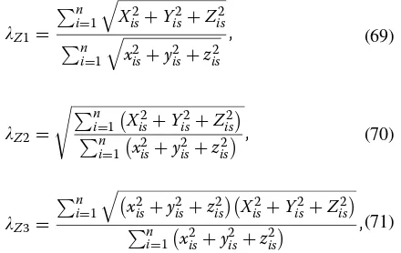
where dxij is coordinate difference of the original points i and j, dx′ij is coordinate difference of the transformed points i and j, H is the scale estimation. Závoti and Kalmár (2016) presented three solutions of scale as follows.
where xis, yis, zis are the centrobaric coordinates in the
original coordinate system, i.e.,
(68)
Case study and discussion Actual case (small rotation angles)
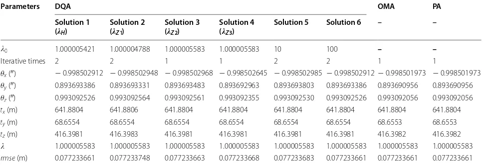
The data are chosen from Grafarend and Awange (2003), and the rotation angles are very small (less than 1′′) in this case. The 3D coordinate of control points in the original system and the target system is listed in Table 2. When the weights of control points are not considered or identical, the computed transformation parameters with presented dual quaternion algorithm (DQA), ortho-normal matrix algorithm (OMA) from Zeng (2015) and Procrustes algorithm (PA) from Grafarend and Awange (2003) are listed in Table 3. DQA sets the threshold τ
to 1.0 × 10⁻¹⁰ and adopts six initial values of , i.e., the solution of Han (2010), the three solutions of Závoti and Kalmár (2016), a biased one (solution 5 with initial value as 10) and a seriously biased one (solution 6 with initial value as 100). From Table 2 it is seen that for the two initial values, i.e., Z2 and Z3, which are identical to the least square estimate, one iterative computation is enough to recover the correct seven transformation parameters. For the rest cases of initial values of , two iterative computation can converge to the correct solu-tion of transformasolu-tion parameters no matter how biased (slightly biased, biased or seriously biased) the initial val-ues of are from best estimate. So DQA converges in two iterations for all situations. OMA and PA have the identi-cal results. From the viewpoint of solution accuracy, the DQA is comparable to the OMA and PA.
At times the weight of the control point needs to be considered because different control points have different accuracy of positioning, and the weight can be obtained based on the different accuracies of the control points. (73)
Table 1 An dual quaternion algorithm of Helmert transformation
Initiation: input 3D coordinates of control points and construct 3D coordinate vector quaternion by Eq. (29), and input the point-wise weight αi, and the initial value =0
Step 1 Compute a, b, c, A, B, C by Eq. (39) to Eq. (44)
Step 2 Compute D by Eq. (61), and carry out the eigenvalue–eigenvector decomposition of D. β1 is set to the largest eigenvalue, and r is set to the eigenvector corresponding to the largest eigenvalue
Step 3 Compute i (subscript i denotes the iterative number) by Eq. (67). If |i−i−1|< τ where τ is a threshold (e.g., 1.0 × 10⁻¹⁰), turn to Step 4, otherwise turn to Step 2 with the value =i
Step 4 Compute R by Eq. (24), furthermore, if rotation angles θx, θy, θz are needed, compute them by Eq. (4). Compute s by Eq. (58) and then t by Eq. (28) and lastly translation t Eq. (26)
Step 5 Compute ei first by substituting solution of r, s, into Eq. (32) and then compute e by Eq. (33). Lastly, compute the root-mean-square error rmse=
e
For the situation that the weight is a point-wise one, i.e., the weight of every point is isotropic for the three axes (x-axis, y-axis, z-axis) directions and control points are independent of each other, the point-wise weight is gen-erated by the means from Grafarend and Awange (2003) and is given in Table 4. The computed results of seven parameters with DQA, OMA and PA are listed in Table 5. For this situation, because the Han (2010) and Závoti and Kalmár (2016) do not consider the weight of con-trol point when computing the solution of scale, all the four solutions (solution 1 to solution 4) just offer slightly biased initial values of . And it is seen from Table 5 that two iterations are needed to obtain the correct result of seven parameters regardless of slightly biased initial value, biased one or seriously biased one. OMA and PA have the identical results if the bias caused by decimal rounding is ignored. From the perspective of computa-tion accuracy, the DQA is consistent with OMA and PA.
Simulative case (big rotation angles)
In this case, the big rotation angles are considered and the data are simulated as follows. The control points and their 3D coordinates in the original system are firstly given in Table 6. Secondly, the true seven transformation
parameters are given in Table 7 with randomly generated big rotation angles. Thirdly, the 3D coordinates of control points in target system are computed by Eq. (1). Lastly, in order to simulate the real-world data which always has noise, the 3D coordinates in the original system are added N(0, 0.022) noise and the 3D coordinates in the tar-get system are added N(0, 0.012) noise. Namely, the case assumes the errors of coordinate in three axes direction equivalent and independent. The normally distributed random noise is produced and listed in Tables 6 and 8.
When the weights of control points are not taken into account or identical, the transformation parameters are computed with DQA, OMA and PA. DQA sets the threshold τ to 1.0 × 10⁻¹⁰ and adopts six initial values
of which are listed in Table 9. DQA requires two itera-tions to obtain the final result for the all six initial values of . And DQA, OMA and PA obtain the identical results which are listed in Table 10.
Furthermore, the performance of DQA, OMA and PA is compared taking into the weights of control points. Firstly, the positional error sphere which is defined from Grafarend and Awange (2003) is calculated and listed in Tables 6 and 8, respectively. And then the point-wise weight matrix is computed by the approach from
Table 2 Coordinates of control points in local system and WGS-84 system
Station name Local system (original system) (m) WGS-84 system (target system) (m)
xo yo zo xt yt zt
Solitude 4,157,222.543 664,789.307 4,774,952.099 4,157,870.237 664,818.678 4,775,416.524 Buoch Zeil 4,149,043.336 688,836.443 4,778,632.188 4,149,691.049 688,865.785 4,779,096.588 Hohenneuffen 4,172,803.511 690,340.078 4,758,129.701 4,173,451.354 690,369.375 4,758,594.075 Kuehlenberg 4,177,148.376 642,997.635 4,760,764.800 4,177,796.064 643,026.700 4,761,228.899 Ex Mergelaec 4,137,012.190 671,808.029 4,791,128.215 4,137,659.549 671,837.337 4,791,592.531 Ex Hof Asperg 4,146,292.729 666,952.887 4,783,859.856 4,146,940.228 666,982.151 4,784,324.099 Ex Kaisersbach 4,138,759.902 702,670.738 4,785,552.196 4,139,407.506 702,700.227 4,786,016.645
Table 3 Computed transformation parameters (identical weight)
Parameters DQA OMA PA
Solution 1 (H)
Solution 2 (Z1)
Solution 3 (Z2)
Solution 4 (Z3)
Solution 5 Solution 6 – –
0 1.000005421 1.000004788 1.000005583 1.000005583 10 100 – –
Iterative times 2 2 1 1 2 2 1 1
θx (″) − 0.998502912 − 0.998502948 − 0.998502968 − 0.998502645 − 0.998502985 − 0.998502912− 0.998501973 − 0.998501973 θy (″) 0.893693386 0.893693331 0.893693483 0.893692963 0.893693803 0.893693386 0.893690956 0.893690956 θz (″) 0.993092526 0.993092564 0.993092561 0.993092355 0.993092530 0.993092526 0.993092056 0.993092056
tx (m) 641.8804 641.8806 641.8804 641.8804 641.8804 641.8804 641.8804 641.8804
ty (m) 68.6554 68.6554 68.6554 68.6554 68.6554 68.6554 68.6553 68.6553
Grafarend and Awange (2003) with the positional error sphere and the recovered transformation parameters (identical weight) as listed in Table 10. The weight result is listed in Table 11 which ignores the magnitude since that ratio of weight rather than absolute weight is more important. Finally, the transformation parameters are computed with DQA, OMA and PA. At this time, DQA
has the same setup of threshold τ and initial values of as that in the identical weight situation. DQA needs two iterations to obtain the final result for the all six initial values of . And DQA, OMA and PA obtain the identical results which are listed in Table 12.
The transformation residuals of coordinates are com-puted by subtracting the calculated coordinates by Eq. (1)
Table 4 Point-wise weight
Station name Solitude Buoch Zeil Hohenneuffen Kuehlenberg Ex Mergelaec Ex Hof Asperg Ex Kaisersbach
Number i 1 2 3 4 5 6 7
αi 2.170137 2.097755 2.208968 2.201671 2.182928 2.268808 2.643404
Table 5 Calculated transformation parameters (point-wise weight)
Parameters DQA OMA PA
Solution 1 (H) Solution 2 (Z1) Solution 3 (Z2) Solution 4 (Z3) Solution 5 Solution 6 – –
0 1.000005421 1.000004788 1.000005583 1.000005583 10 100 – –
Iterative times 2 2 2 2 2 2 1 1
θx (″) − 0.997716767 − 0.997716882 − 0.997716767 − 0.997716882 − 0.997716767 − 0.997716767 − 0.997716185 − 0.997716186
θy (″) 0.896086322 0.896087012 0.896086322 0.896087012 0.896086322 0.896086322 0.896085615 0.896085615
θz (″) 0.985885473 0.985885475 0.985885473 0.985885475 0.985885473 0.985885473 0.985885069 0.985885070
tx (m) 641.8395 641.8395 641.8395 641.8395 641.8395 641.8395 641.8395 641.8395
ty (m) 68.4729 68.4729 68.4729 68.4729 68.4729 68.4729 68.4729 68.4729
tz (m) 416.2155 416.2155 416.2155 416.2155 416.2155 416.2155 416.2156 416.2156
1.000005611 1.000005611 1.000005611 1.000005611 1.000005611 1.000005611 1.000005611 1.000005611 rmse (m) 0.114082157 0.114082183 0.114082157 0.114082183 0.114082157 0.114082157 0. 114082157 0.114082157
Table 6 3D coordinates of control points in original system and noises added (m)
Point no. xo
yo
zo
Noise in xo
Noise in yo
Noise in zo
Positional error sphere
1 10.00000 30.00000 5.00000 − 0.03190 0.02380 0.01060 0.00057
2 20.00000 30.00000 12.50000 − 0.02880 − 0.02400 0.00440 0.00047
3 30.00000 30.00000 15.00000 0.01140 − 0.00040 − 0.01840 0.00016
4 10.00000 20.00000 9.50000 − 0.00800 − 0.00310 − 0.04340 0.00065
5 20.00000 20.00000 11.00000 0.01380 − 0.03210 − 0.00120 0.00041
6 30.00000 20.00000 10.00000 0.01630 0.00510 − 0.02020 0.00023
7 10.00000 10.00000 14.50000 0.01420 − 0.02110 0.01230 0.00027
8 20.00000 10.00000 4.50000 0.02580 0.02830 0.01020 0.00052
9 30.00000 10.00000 4.00000 0.01340 − 0.01610 0.03380 0.00053
Table 7 True values of transformation parameters
tx (m) ty (m) tz (m) θx (°) θy (°) θz (°)
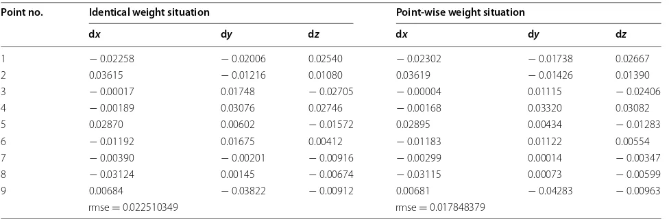
with the recovered transformation parameters and coor-dinates in the source system to known coorcoor-dinates in the target system. The result is listed in Table 13, where dx , dy and dz denote the transformation residuals of
coor-dinates in the three axes direction. And the root-mean-square errors are also computed and listed in Table 13. It is seen from Table 13 that the transformation residuals of coordinates are consistent with the noises added into coordinates of control points in the original system.
According to the above analysis, DQA, OMA and PA have the identical performance for the big rotation angles. Thus, the presented algorithm is correct and reliable.
Conclusions
Unit dual quaternion can be elegantly employed to describe the rigid transformation including rotation and translation. Based on unit dual quaternion, a non-differential model of Helmert transformation (seven-parameter similarity transformation) is constructed and a rigid iterative algorithm of Helmert transfor-mation using dual quaternion is presented. The case study shows the presented algorithm requires one iteration to recover the transformation parameter if accurate initial value of scale is provided like the solu-tions no. 2 and 3 of Závoti and Kalmár (2016) for the situation that the weights are identical; otherwise,
Table 8 3D coordinates of control points in target system and noises added (m)
Point no. xt yt zt Noise in xt Noise in yt Noise in zt Positional error sphere
1 51.20845 10.62821 37.12165 0.00800 0.00390 − 0.00270 0.00003
2 52.95745 15.95030 48.29655 0.00940 0.00090 − 0.01190 0.00008
3 54.22132 16.38806 58.51758 − 0.00990 − 0.00640 − 0.02200 0.00021
4 41.74440 15.77468 39.17225 0.00210 − 0.00560 0.00990 0.00004
5 42.91124 15.23557 49.20249 0.00240 0.00440 − 0.00520 0.00002
6 43.83551 12.25430 58.75580 − 0.01010 − 0.00950 0.00330 0.00007
7 32.32886 21.40958 41.31824 − 0.00740 0.00780 0.00230 0.00004
8 32.37989 9.63651 49.15455 0.01080 0.00570 0.00020 0.00005
9 33.35267 7.14367 58.80324 − 0.00130 − 0.00820 − 0.01000 0.00006
Table 9 Six initial values of scale parameter
Solution 1 (H) Solution 2 (Z1) Solution 3 (Z2) Solution 4 (Z3) Solution 5 Solution 6
0.99957261825858 0.99966151537312 0.99951849936829 0.99951723170141 10 100
Table 10 Recovered transformation parameters (identical weight) by DQA (with six initial values of scale parameter), OMA and PA
tx (m) ty (m) tz (m) θx (°) θy (°) θz (°)
20.030886056 10.008832821 29.984374281 31.779990101 76.995092442 63.207363719 0.999514725
Table 11 Point-wise weight
Point no. i 1 2 3 4 5 6 7 8 9
αi 0.5561 0.6066 0.9013 0.4835 0.7759 1.1119 1.0762 0.5853 0.5655
Table 12 Recovered transformation parameters (point-wise weight) by DQA (with six initial values of scale parameter), OMA and PA
tx (m) ty (m) tz (m) θx (°) θy (°) θz (°)
exact two iterative computation converges to the cor-rect solution of transformation parameters no matter how big the rotation angles are and how biased the ini-tial value of scale is. Hence, the presented algorithm has an excellent or fast convergence, and it becomes an analytical algorithm when the accurate initial value of scale is offered. In addition, the presented algorithm is able to deal with point-wise weight transformation which is more rational than those algorithms which do not consider the weight difference among control points. And from the viewpoint of solution accuracy, the presented algorithm is comparable to the classic Procrustes algorithm and orthonormal matrix algo-rithm from Zeng (2015).
Authors’ contributions
HZ carried out the theoretic studies including establishing the Helmert trans-formation model using dual quaternion, deriving the solution of transforma-tion parameters by Lagrangian extremum law and designing the case study, additionally drafted the manuscript. XF conceived of the study and helped to draft the manuscript. GC participated in deriving the solution of transforma-tion parameters. RY carried out the case computatransforma-tion and performed case analysis. All authors read and approved the final manuscript.
Author details
1 Key Laboratory of Geological Hazards on Three Gorges Reservoir Area, Ministry of Education, China Three Gorges University, Yichang 443002, China. 2 Hubei Key Laboratory of Intelligent Vision Based Monitoring for Hydro-electric Engineering, China Three Gorges University, Yichang 443002, China. 3 Hubei Key Laboratory of Construction and Management in Hydropower Engineering, China Three Gorges University, Yichang 443002, China. 4 School of Geodesy and Geomatics, Wuhan University, Wuhan 430079, China. 5 School of Environmental Science and Spatial Informatics, China University of Mining and Technology, Xuzhou 221116, China. 6 School of Civil Engineering, Chong-qing University, ChongChong-qing 400030, China. 7 Chongqing Survey Institute, Chongqing 401121, China.
Acknowledgements
The study is supported jointly by Hubei Provincial Natural Science Foundation of China (Grant No. 2016CFB443), the Open Foundation of the Key Laboratory of Precise Engineering and Industry Surveying, National Administration of Surveying, Mapping and Geoinformation of China (Grant No. PF2015-14), the 2015 Open Foundation of Hubei Key Laboratory of Intelligent Vision Based Monitoring for Hydroelectric Engineering, China Three Gorges University (Grant No. 2015KLA06), the Open University Teaching Research Project of China Three Gorges University (Grant No. KJ2015019), the Open Foundation of Hubei Key Laboratory of Construction and Management in Hydropower Engineering, China Three Gorges University (Grant No. 2014KSD13) and National Natural Science Foundation of China (Grant No. 41774009, 41774005, 41104009). The first author is grateful to Professor Daniel Chaney for polishing the English of the paper. Last but not the least, the author’s special thanks are given to Dr. Thomas Hobiger and two anonymous reviewers for their valuable comments and suggestions, which enhance the quality of this manuscript.
Ethics approval and consent to participate Not applicable.
Competing interests
The authors declare that they have no competing interests.
Availability of data and materials
The actual case data are collected from Grafarend and Awange (2003). In the simulative case, the 3D coordinates of control points in the target system are produced given the 3D coordinates in the original system and the seven transformation parameters.
Appendix 1: Proof of symmetric property of matrix A
Substituting Eq. (29) into Eqs. (17) and (16) gives
(74) W(poi)=
0 zoi −yoi xoi
−zio 0 xoi yoi yoi −xoi 0 zio −xoi −yoi −zoi 0
,
(75)
Q(pti)=
0 −zti yti xti zti 0 −xti yti
−yti xit 0 zit
−xti −yti −zti 0 ,
Table 13 Transformation residuals of coordinates (m)
Point no. Identical weight situation Point-wise weight situation
dx dy dz dx dy dz
1 − 0.02258 − 0.02006 0.02540 − 0.02302 − 0.01738 0.02667
2 0.03615 − 0.01216 0.01080 0.03619 − 0.01426 0.01390
3 − 0.00017 0.01748 − 0.02705 − 0.00004 0.01115 − 0.02406
4 − 0.00189 0.03076 0.02746 − 0.00168 0.03320 0.03082
5 0.02870 0.00602 − 0.01572 0.02895 0.00434 − 0.01283
6 − 0.01192 0.01675 0.00412 − 0.01183 0.01122 0.00554
7 − 0.00390 − 0.00201 − 0.00916 − 0.00299 0.00014 − 0.00347
8 − 0.03124 0.00145 − 0.00674 − 0.03115 0.00073 − 0.00599
9 0.00684 − 0.03822 − 0.00912 0.00681 − 0.04283 − 0.00963
thus
Aktuğ B (2012) Weakly multicollinear datum transformations. J Surv Eng 138(4):184–192
Akyilmaz O (2007) Total least squares solution of coordinate transformation. Surv Rev 39(303):68–80
Arun KS, Huang TS, Blostein SD (1987) Least-squares fitting of two 3-D point sets. IEEE Trans Pattern Anal Mach Intell 9:698–700
Burša M (1967) On the possibility of determining the rotation elements of geodetic reference systems on the basis of satellite observations. Stud Geophys Geod 11(4):390–396
Chang G (2015) On least-squares solution to 3D similarity transformation prob-lem under Gauss–Helmert model. J Geod 89:573–576
Chang G, Xu T, Wang Q, Zhang S, Chen G (2017) A generalization of the analytical least-squares solution to the 3D symmetric Helmert coordinate transformation problem with an approximate error analysis. Adv Space Res 59:2600–2610
Chen Y, Shen YZ, Liu DJ (2004) A simplified model of three dimensional-datum transformation adapted to big rotation angle. Geomat Inf Sci Wuhan Univ 29(12):1101–1105
El-Habiby MM, Gao Y, Sideris MG (2009) Comparison and analysis of non-linear least squares methods for 3-D coordinates transformation. Surv Rev 41(311):26–43
El-Mowafy A, Fashir H, Al-Marzooqi Y (2009) Improved coordinate transforma-tion in Dubai using a new interpolatransforma-tion approach of coordinate differ-ences. Surv Rev 41(311):71–85
Grafarend EW, Awange JL (2003) Nonlinear analysis of the three-dimensional datum transformation[conformal group C7(3)]. J Geod 77:66–76 Han JY (2010) Noniterative approach for solving the indirect problems of linear
reference frame transformations. J Surv Eng 136(4):150–156 Han JY, Van Gelder HWB (2006) Step-wise parameter estimations in a
time-variant similarity transformation. J Surv Eng 132(4):141–148
Horn BKP (1986) Robot Vision. MIT Press. McGraw-Hill, Cambridge, New York Horn BKP (1987) Closed-form solution of absolute orientation using unit
quaternions. J Opt Soc Am Ser A 4:629–642
Horn BKP, Hilden HM, Negahdaripour S (1988) Closed-form solution of absolute orientation using orthonormal matrices. J Opt Soc Am Ser A 5:1127–1135
Jaw JJ, Chuang TY (2008) Registration of ground-based LIDAR point clouds by means of 3D line features. J Chin Inst Eng 31(6):1031–1045
Jitka P (2011) Application of dual quaternions algorithm for geodetic datum transformation. Aplimat J Appl Math 4(2):225–236
Kashani I (2006) Application of generalized approach to datum transformation between local classical and satellite-based geodetic networks. Surv Rev 38(299):412–422
Krarup T (1985) Contribution to the geometry of the Helmert transformation. Geodetic Institute, Denmark
Leick A (2004) GPS satellite surveying, 3rd edn. Wiley, Hoboken
Leick A, van Gelder BHW (1975) On similarity transformations and geodetic network distortions based on Doppler satellite observations. Rep. No. 235, Department of Geodetic Science, Ohio State University, Columbus, Ohio
Mikhail EM, Bethel JS, McGlone CJ (2001) Introduction to modern photogram-metry. Wiley, Chichester
Neitzel F (2010) Generalization of total least-squares on example of weighted 2D similarity transformation. J Geod 84(12):751–762. https://doi. org/10.1007/s00190-010-0408-0
Springer Nature remains neutral with regard to jurisdictional claims in pub-lished maps and institutional affiliations.
Received: 18 September 2017 Accepted: 29 January 2018
References
Paláncz B, Awange JL, Völgyesi L (2013) Pareto optimality solution of the Gauss–Helmert model. Acta Geod Geophys 48:293–304
Shen YZ, Hu LM, Li BF (2006a) Ill-posed problem in determination of coordi-nate transformation parameters with small area’s data based on Bursa model. Acta Geod Cartogr Sin 35(2):95–98
Shen YZ, Chen Y, Zheng DH (2006b) A quaternion-based geodetic datum transformation algorithm. J Geod 80:233–239
Soler T (1998) A compendium of transformation formulas useful in GPS work. J Geodyn 72(7–8):482–490
Soler T, Snay RA (2004) Transforming positions and velocities between the International Terrestrial Reference Frame of 2000 and North American Datum of 1983. J Surv Eng 130(2):49–55
Soycan M, Soycan A (2008) Transformation of 3D GPS Cartesian coordinates to ED50 using polynomial fitting by robust re-weighting technique. Surv Rev 40(308):142–155
Teunissen PJG (1986) Adjusting and testing with the models of the affine and similarity transformation. Manuscr Geod 11:214–225
Teunissen PJG (1988) The non-linear 2D symmetric Helmert transformation: an exact non-linear least-squares solution. Bull Géod 62:1–16
Walker MW, Shao L, Volz RA (1991) Estimating 3-D location parameters using dual number quaternions. CVGIP Image Underst 54:358–367 Wang YB, Wang YJ, Wu K, Yang HC, Zhang H (2014) A dual quaternion-based,
closed-form pairwise registration algorithm for point clouds. ISPRS J Photogramm Remote Sens 94:63–69
Xu PL (2002) A hybrid global optimization method: the one-dimensional case. J Comput Appl Math 147:301–314
Xu PL (2003a) A hybrid global optimization method: the multi-dimensional case. J Comput Appl Math 155:423–446
Xu PL (2003b) Numerical solution for bounding feasible point sets. J Comput Appl Math 156:201–219
Závoti J, Kalmár J (2016) A comparison of different solutions of the Bursa–Wolf model and of the 3D, 7-parameter datum transformation. Acta Geod Geophys 51:245–256
Zeng HE (2014) Planar coordinate transformation and its parameter estimation in the complex number field. Acta Geod Geophys 49(1):79–94
Zeng HE (2015) Analytical algorithm of weighted 3D datum transformation using the constraint of orthonormal matrix. Earth Planets Space 67:105. https://doi.org/10.1186/s40623-015-0263-6
Zeng HE, Huang SX (2008) A kind of direct search method adopted to solve 3D coordinate transformation parameters. Geomat Inf Sci Wuhan Univ 33(11):1118–1121
Zeng WX, Tao BZ (2003) Non-linear adjustment model of three-dimensional coordinate transformation. Geomat Inf Sci Wuhan Univ 28(5):566–568 Zeng HE, Yi QL (2010) A new analytical solution of nonlinear geodetic datum
transformation. In: Proceedings of the 18th international conference on geoinformatics
Zeng HE, Yi QL (2011) Quaternion-based iterative solution of three-dimen-sional coordinate transformation problem. J Comput 6(7):1361–1368 Zeng HE, Yi QL, Wu Y (2016) Iterative approach of 3D datum transformation