R E S E A R C H
Open Access
Source localization and tracking in a dispersive
medium using wireless sensor network
Kamrul Hakim
*and Sudharman K Jayaweera
Abstract
In this paper, we address the issue of collaborative information processing for diffusive source localization and tracking using wireless sensor networks capable of sensing in dispersive medium/environment. We first determine the space-time concentration distribution of the dispersion from physical modeling and mathematical formulations of an underwater oil spill scenario, considering the effect of laminar water velocity as an external force. For static diffusive source localization, we propose two parametric estimation techniques based on maximum-likelihood (ML) and best linear unbiased estimator for the special case of our physical dispersion model. We prove the consistency and asymptotic normality of the obtained ML solution when the number of sensor nodes and samples approach infinity, and derive the Cramér-Rao lower bound on its performance. We also propose a particle filter-based target tracking scheme for moving diffusive source and derive the posterior Cramér-Rao lower bound for the moving source state estimates as a theoretical performance bound. The performance of the proposed schemes are shown through numerical simulations and compared with the derived theoretical bounds.
Keywords: Wireless sensor network; Diffusion; Source localization; Tracking; Parameter estimation; Maximum-likelihood; Best linear unbiased estimator; Particle filter
1 Introduction
The release of liquid petroleum hydrocarbon into the ocean or coastal water due to human activity has attracted tremendous attention because of its environmental, bio-logical, and economical impact. Recent BP oil disaster in the Gulf of Mexico is a perfect example of how spill stemmed from a sea-floor oil gusher can severely dam-age the marine and wildlife habitats as well as the Gulf ’s fishing and tourism industries. Research in modeling and predicting the extent of such oil spill can assist in plan-ning and emergency decision-making, thereby reducing the threats and hazardous effects on the environment as well as the economic cost. Considering the fact that this is a diffusive source estimation and tracking problem, such research can in general be applicable in many other similar contexts such as homeland security, environmental and industrial monitoring, pollution control, servers, and data center temperature monitoring as well [1-8]. For example,
*Correspondence: [email protected]
Department of Electrical and Computer Engineering, University of New Mexico, Albuquerque, NM 87131-0001, USA
the spread of chemical and biological agents as homeland security problems are discussed in [5,9-11].
Recent advances in sensor technology, such as smart/intelligent nodes with cognitive abilities, on-board sensors, and wireless networking capabilities have trig-gered the use of wireless sensor networks (WSNs) in monitoring various physical phenomena [12-14]. Though sensor nodes are capable of a limited amount of local processing and wireless communication, when a large number of sensors communicate and share informa-tion among themselves, they can measure a desired phenomenon-of-interest in great detail. Also with the developments of unmanned autonomous vehicles, WSNs are gaining popularity due to their potential to be useful for a wide range of applications including environmental monitoring, intrusion detection, and various military and civilian applications [12,15,16]. Due to advanced micro-electromechanical systems, many of the state-of-the-art sensors are now more accurate, robust against noise, and energy efficient [17,18]. These new cutting-edge sensors can withstand severe unfavorable conditions in hazardous areas where human deployment is impossible. All these useful and exciting features in recently developed sensors
make them suitable candidates for the set of applications involving monitoring of diffusion phenomena that we are interested in.
Source or target localization using distributed sensor arrays is an area of active research interest for a consid-erable period of time [19,20]. In the past, detection and localization problems of diffusive sources in WSN have been a topic of interest, specially in the case of chemi-cal/biological threat detection. Interesting research in this context can be found in [3,4,9,10], where biochemical con-centration distribution in space and time for different types of diffusive sources, diffusion models, and/or sensor networks is estimated. For instance, remotely localizing a gas or odor source using mobile robot was proposed in [3] by fitting the gas distribution model to the gas sen-sor response at the sensen-sor locations. However, the mobile sensor dynamics model therein was obtained empirically, which does not allow for dynamic environment and mov-ing diffusive source. In [4], a maximum-likelihood (ML) estimator was developed for localizing vapor-emitting sources, and its asymptotic normality of the obtained ML estimator was proved when the signal-to-noise-ratio (SNR) approaches infinity. Many other estimation tech-niques have also been used in diffusive source parameters estimation literature [9,10,21-23]. In particular, Bayesian estimation has been applied in [9,21] in a sequential man-ner, which is not suitable in many practical scenarios where faster estimation and immediate actions based on the estimation are top priorities. A real-time maximum-likelihood estimation method was proposed in [23] for estimating diffusive source parameters, where consistency and asymptotic efficiency of the obtained estimator were proved when the density of sensors becomes infinite. In [24], the problem of impulsive diffusive source localiza-tion was solved assuming the spatial sensor measurements at any sensor location as a scaled and shifted version of a common prototype function, leading to solving a set of linear equations. However, the physical diffusion models used in [23,24] are oversimplified with the diffu-sive sources assumed to be impuldiffu-sive or instantaneous in nature.
Although research has been done in tracking and/or estimating time-varying parameter estimation in gen-eral [25-28], to the best of our knowledge, very few attempts have been made in time-varying diffusive source parameter estimation. Some of these methods cannot be applied directly into our time-varying parameter estima-tion model since, e.g., for a moving source, the concen-tration at the current time is affected by all past values of source position. Therefore, time-cumulation effects on the concentrations (i.e., observations) must be taken into account to estimate time-varying parameters. Among previous works, a parametric moving path model for a diffusive moving source was discussed in [10], where
the moving source path was approximated using finite number basis functions. Tracking performance in this case depends on the smoothness of the source trajectory, prior information about the moving source trajectory, and choosing a suitable finite set of basis functions. In [29], a novel recursive algorithm was proposed to track the inten-sity of a diffusive point source, but the source location was considered as an unknown static value.
The aforementioned limitations may be overcome by developing or exploiting state-of-the-art Bayesian-based location tracking methods suitable for handling highly nonlinear diffusion processes. In the Bayesian approach, the key is to construct the posterior probability density function (PDF) of the underlying state vector based on all available information. For linear and Gaussian state dynamics and observation models, the optimal minimum mean squared error (MMSE) solution is tractable and is given by the well-known Kalman filter [30]. However, for most of the real-world scenarios, dynamic state estimation problems are nonlinear and non-Gaussian, and obtaining optimal closed-form solution is not tractable under the Bayesian approach. In these cases, suboptimal approaches such as extended Kalman filter and Gaussian-sum filter [31] are used with certain approximations. These sub-optimal algorithms become inefficient for highly nonlin-ear and non-Gaussian systems. In these cases, numerical techniques based on sequential Monte Carlo methods are used to achieve better performance for highly nonlinear systems. To that end, the idea of particle filtering was introduced in [32] as an effective method of representing PDF in terms of a set of random sampling.
To the best of our knowledge, moving diffusive source tracking using particle filtering approach has not been attempted before. The posterior Cramér-Rao lower bound (PCRLB) for the moving source state estimates is also derived as a theoretical performance bound [34].
The remainder of this paper is organized as follows: Sections 2 and 3 discuss, respectively, modeling of an underwater oil spill scenario and measurement model for static diffusive source localization using sensor net-work. The proposed statistical methods for static diffusive source localization and corresponding theoretical per-formance bound are discussed in Section 4. Section 5 presents the proposed particle filter-based method for moving diffusive source tracking with theoretical per-formance bound analysis in detail. Section 6 shows the validity and effectiveness of our proposed methods for diffusive source localization and tracking through numer-ical simulations. Finally, Section 7 concludes the paper by summarizing our results.
2 Physical model for dispersion
We first derive the physical models for the space-time sub-stance dispersion mechanisms from a diffusive source and then transform the obtained dispersion model to a statis-tical measurement model. The transport model of a sub-stance from a diffusive source can be obtained by solving the corresponding diffusion equation. Diffusion equation describes the dispersion of particles from a region of high concentration to regions of lower concentration due to random molecular motion. Let us denote the concentra-tion of the diffused substance at a posiconcentra-tionr = [x,y,z]T and at time t as c(r, t). Ignoring the effects of external forces for a source-free volume and for space-invariant diffusivity constant κ, the concentration of a dispersed substance follows the following diffusion equation [35]:
∂c(r,t)
∂t =κ
∂2c(r,t)
∂x2 +
∂2c(r,t)
∂y2 +
∂2c(r,t) ∂z2
.
To solve the above differential equation, appropriate boundary and initial conditions are required. We first compute the concentration for a stationary impulse point source of unit mass to obtain Green’s function. The obtained result is then extended for a continuous source by integrating the source-release rate with the Green’s function. Denoting the Green’s function of the impulse source ascG(r,t), the concentration of a continuous point source with mass release rateμ(t)and initial release time tIcan then be given by the following integral:
c(r,t)= t
tI
μ(τ )cG(r,t−τ )dτ. (1)
For parametric estimation case, it is to be noted that from the concentration measurements taken by the sen-sors, we can first estimate the source parameters of inter-est and then predict its cloud evolution in space and time by inserting the estimated parameters into (1).
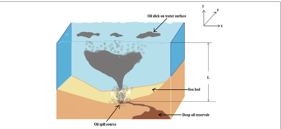
Although the main focus of this paper are diffusive source localization and tracking, we introduce a special diffusion phenomenon, i.e., an underwater oil spill, to demonstrate how to model and solve for a practical dif-fusion phenomenon and also to motivate the practical importance of the problem we are discussing. As shown in Figure 1, we model an underwater oil spill as a diffu-sion occurring in a two-layer semi-infinite medium (i.e., water and air). We assume that the oil spilling source is located at the bottom (i.e., river/sea bed) at a loca-tion r0 =[x0,y0,z0]T. The depth of water level is 0 ≤ z≤Lwith diffusivityκwand concentrationcw. The same
quantities for air (z>L) are denoted asκaandca
respec-tively. Along the z-axis, we need to solve the following differential equations:
∂cw ∂t =κw
∂2cw
∂z2 , for 0<z<L, ∂ca
∂t =κa ∂2ca
∂z2, forz>L.
Considering only point impulse source located atz=z0, where 0 ≤ z0 ≤ Land impermeable boundary atz = 0, we have the following initial condition:
cw(z,t)=δ(z−z0), at t=tI and boundary conditions
cw=ca, atz=L, (2)
κw ∂cw
∂z =κa ∂ca
∂z , atz=L, (3)
∂cw
∂z =0, atz=0. (4)
spatio-Figure 1An underwater oil spill scenario.
temporal concentration distribution (omitting the details in [10,35,36]):
cw(z,t)=
1 2√π κw(t−tI)
∞
n=0 ρn
exp
−(z−z0−2nL)2 4κw(t−tI)
+exp
−(z+z0+2nL)2 4κw(t−tI)
+ 1
2√π κw(t−tI) ∞
n=0 ρ(n+1)
×
exp
−(z−z0−2(n+1)L)2 4κw(t−tI)
+exp
−(z+z0+2(n+1)L)2 4κw(t−tI)
,
whereρ =
√
κw−√κa
√
κw+√κa. As can be seen, the concentration
curve can be considered to be the superimposed curve resulting from each successive reflection (from the sur-face layer) being superimposed on the original curve. In practice, ifκwκa, thenρ→1. Therefore we have,
cw(z,t)=
1 2√π κw(t−tI)
exp
− (z−z0)2 4κw(t−tI)
+exp
− (z+z0)2 4κw(t−tI)
+ √ 1
π κw(t−tI)
∞
n=1
exp
−(z−z0−2nL)2 4κw(t−tI)
+exp
−(z+z0+2nL)2 4κw(t−tI)
.
(5)
Considering the laminar water velocity working along the X-Y-plane as an external force, we have v = [vx,vy, 0]T. The diffusion equations along thexandyaxes
will include additionaladvectionterm [35]:
∂cw ∂t =κw
∂2cw ∂x2 −vx
∂cw ∂x, ∂cw
∂t =κw ∂2cw
∂y2 −vx ∂cw
∂y.
ForX-Y-plane, there is no boundary condition and the initial condition is given as
c(x,y,t)=δ(x−x0,y−y0), att=tI.
Using the concept of Fourier transform for solving par-tial differenpar-tial equations, we can solve for the following concentration distribution alongxandyaxes [37]:
cw(x,t)=
exp−{x−x0−vx(t−tI)}2 4κw(t−tI)
2√π κw(t−tI)
and (6)
cw(y,t)=
exp−{y−y0−vy(t−tI)}2 4κw(t−tI)
2√π κw(t−tI)
. (7)
concentration distribution can be obtained as the product dering the source mass release rate to be constantμ(t)= μ, the final solution for concentration of oil diffusion in water for stationary continuous source with mass rate of
μ(t)can be obtained from (1):
Derivation to (9) is given in Appendix 1. For the sake of simplicity from here on, we denote the diffusivity constant
κw=κ.
2.1 Moving diffusive source
For a moving diffusive source-emitting substance con-tinuously in a semi-infinite medium similar to our case, space-time concentration distribution can be obtained using the concept of convolution integral from the Green’s function solution corresponding to stationary impulsive source. In this case, substance concentration at any time instant is affected by all the past values of source posi-tion and release rate. Therefore, time-cumulaposi-tion effect on the concentrations has to be considered to obtain complete physical model. For a moving diffusive source continuously releasing substance at a mass rateμ(t), the space-time concentration distribution in a semi-infinite medium can be obtained for a given Green’s function cG(r,t)using the following integral: moving path. The advantage of solving the physical dif-fusion model corresponding to a moving diffusive source using (10) is that the initial, boundary, and other neces-sary conditions can be taken into account to solve for the stationary case in the first step before extending it to the moving source case.
3 Measurement and system models for static diffusive source localization
We consider a WSN consisting of a fusion center (FC) and N spatially distributed biochemical static sensor nodes capable of sensing in dispersive environment. For prac-tical consideration, we assume that the N distributed sensors are located in a rectangular volume in space such thatrj = [xj,yj,zj]T∈ ,∀j ∈ {1, 2,. . .,N}, where =
[a1,a2]×[b1,b2]×[c1,c2] ⊆ R3. It is also assumed that the source-to-sensor distances are much higher than the source and sensor dimensions. Each sensor node takes measurements at times tk;∀k ∈ {1, 2,. . .,T}, where T
is the total number of time samples. Assuming that the physical model discussed before is the underlying disper-sion mechanism, we may obtain a measurement model for a sensor at a positionrj and at timetk asy(rj,tk) = c(rj,tk)+e(rj,tk)+b, wherec(rj,tk)is the concentration
of interest,bis a bias term, ande(rj,tk)∼N(0,σ2)is the
sensor noise assumed to be independent in both time and space. For the sake of brevity, it can be rewritten in the simplified form as
where yj,k = y(rj,tk), ej,k = e(rj,tk), cj,k(θ) = c(rj,tk),
θ ∈Rn×1is the unknown source and medium parameter vector that we are interested to estimate, andbis the bias or clutter term representing the sensor’s response to for-eign substances that may be present in a diffusive field of interest. The bias term is assumed to be space and time-invariant such that the foreign substances interfering with the actual measurements are in steady state. If we want to localize a static diffusive source, then only [x0,y0,z0] are the parameters of interest. It is to be noted that some of the parameters, such as the diffusivity constantκ, bias termb, and noise varianceσ2, can be measured at the cal-ibration stage, thereby reducing the cost of computation during the detection/estimation phase.
We assume that the sensor nodes are in sleep mode until they are activated by some central control (i.e., FC) due to a possible release of a substance from a diffusive source. The activated sensor nodes take measurements of the sub-stance’s concentration at time instantstks and then return to sleep mode. For N number of nodes in a WSN and with each node takingT number of time samples of the substance concentrations at their respective locations, let y∈RNT×1be the measurement vector received at the FC.
4 Static diffusive source localization
In this section, we use the maximum-likelihood estima-tor (MLE) and the BLUE to estimate the location of an underwater diffusive source diffusing oil into water. For simplicity of exposition, we consider a special case of our obtained physical model when an oil spill occurs in an infinite (L → ∞) underwater medium. In this case, the concentration at any positionrjat timetkis reduced to the
following expression [4,35]:
cj,k(θ)= μ
4π κ|rj−r0| erfc
| rj−r0| 2√κ(tk−tI)
. (12)
where erfc(.)is the complementary error function.
4.1 Maximum-likelihood-based source localization
From the measurement model discussed in Section 3, the conditional PDF of the measurements taken by the jth node at timetkisp(yj,k|θ)∼N(cj,k(θ)+b,σ2). Hence, the
log-likelihood function formed at the FC can be written as
L= −NT
2 log(2π σ 2)− 1
2σ2 N
j=1 T
k=1
yj,k−cj,k(θ)−b 2
.
(13)
The log-likelihood equations are obtained by ∂ci∂(,jθ(θ)):
N
j=1 T
k=1
yj,k−cj,k(θ)−b
∂cj,k(θ)
∂θu
θ=ˆθ
=0, (14)
foru=1, 2, 3, whereθuis theuth element ofθ, and ∂cj,k(θ)
∂θu =
μrj(u)−r0(u)
4π κ|rj−r0|2 ⎡ ⎣erfc
|r j−r0| 2√κ(tk−tI)
|rj−r0|
+exp
− |rj−r0|2 4κ(tk−tI)
√
π κ(tk−tI) ⎤ ⎥
⎦. (15)
Since the system of equations in (14) is nonlinear, there is no closed-form solution to it. We can obtain an ML esti-mation of the source location using any suitable nonlinear optimization technique. In this case, (14) is solved using simplex search algorithm [38].
The CRLB provides a lower limit on the mean squared estimation error of an unbiased estimator of nonrandom parameter [30]. CRLB in this case can be obtained as CRLB ≥ I−θ1, whereIθ ∈ R3×3is the Fisher information matrix (FIM) formed at the FC. Theu-vth element of the FIM can be found as
[Iθ]u,v=E
∂ ∂θu
logp(y|θ) ∂ ∂θv
logp(y|θ) ,
= 1
σ2 N
j=1 T
k=1 ∂
cj,k(θ) ∂θu
∂cj,k(θ)
∂θv
, (16)
where (16) was obtained using the independence assump-tion of observaassump-tions in space and in time.
A sequence of estimatorsθˆnto an unknown parameter
vectorθ is said to be consistent if the sequence converges in probability to θ, i.e., limn→∞θˆn = θ, wheren is the
sample size [30]. It is desirable to have a consistent MLE as consistency ensures that for large data sets, the MLE will converge to the true parameter. The obtained MLE to our source localization problem is consistent when the number of sensor nodes in any non-negligible open sub-set of = [a1,a2]×[b1,b2]×[c1,c2] ⊆ R3 and time samples go to infinity.
Theorem 1. If the number of sensors N increases
in such a way that for any open subset =
[a1,a2]×[b1,b2]×[c1,c2] ⊆ R3having positive area, the number of sensors N and/or the number of time samples T tend to infinity, the obtained ML estimator is consistent.
Proof. See Appendix 2.
Once consistency for the obtained MLE is established, the next important thing is to check the asymptotic nor-mality. An asymptotically normal estimator is a consistent estimator whose distribution around the true parameter θ approaches a normal distribution with standard devia-tion shrinking in propordevia-tion to 1/√nas the sample sizen grows, i.e.,√nIθ
ˆ θn−θ
are the Fisher information and identity matrices, respec-tively [30]. It ensures that the estimator not only converges to the unknown parameter, but it converges fast enough at a rate 1/√n. We address this issue with the following theorem on asymptotic normality.
Theorem 2. If the number of sensors N and time samples T increase as in Theorem 1, then for a true parameter vec-tor θ0 ∈ ◦, where ◦ ⊂ is an open subset of , the following is true:
√ NT
ˆ
θMLy−θ0
−→N0,¯Iθ0
−1 ,
in distribution where the(u,v)th element of the matrixI¯θ is given by
¯ Iθ
u,v=N,limT→∞
1
σ2NT N
j=1 T
k=1 ∂c
j,k(θ) ∂θu
∂cj,k(θ) ∂θv
.
Proof.See Appendix 3.
4.2 Best linear unbiased estimator-based source localization
The advantages of using the BLUE for static diffusive source localization are that there are no constraints on the PDF and also knowing only the mean and covariance of the measurements is enough. However, observations have to be linear for the BLUE algorithm. In this subsection, we assume that the distributed sensing nodes are capable of estimating their respective distances from the source using BLUE.
Since the complementary error function can be approx-imated as erfc(z) ≈ 1− √2
πz, our observation model for jth node at thekth time instant can be linearized in terms of the inverse of the source-to-node distances from (11) and (12):
yj,k≈
μ|rj−r0|−1 4π κ +
b− μ
4π3κ3(tk−tI)
+ej,k
=hdinvj +ak+ej,k,
(17)
where h = 4π κμ , djinv = rj−r0−1 and ak = b − μ
4√π3κ3(tk−tI). Since all the parameters are known except for the diffusive source location, we can write˜yj,k=yj,k− ak=hdjinv+ej,k. Therefore, the observation vector formed
at thejth node can be written as
˜ yj =
⎛ ⎜ ⎜ ⎜ ⎝
yi1−a1 yi2−a2
.. . yiT−aT
⎞ ⎟ ⎟ ⎟
⎠=hdinvj +ej, (18)
where h is a column vector of all hs and ej =
[ei1,ei2,. . .,eiT]T. Since ej,k ∼ N
0,σ2 for ∀j,k and measurement noise is assumed to be independent and identically distributed across space and time, the covari-ance matrix of y˜j is ˜j = diag
σ2,σ2,. . .,σ2 ∈
RT×T. The optimal BLUE estimator formed atjth node is
given by
ˆ djinv= h
T˜−1 j y˜j
hT˜j−1h, (19)
with estimator varianceVj=
hT˜j−1h −1
.
After the distributed nodes estimate their respective distancesdˆj = |rj−r0|from the source using BLUE, all nodes senddˆjs to the FC for further processing. It is to
be noted that the source-to-node distance estimation can also be performed at the FC. The signal received at the FC from thejth node can be expressed asfj= ˆdj+wj, where wjis normally distributed with mean 0 and varianceσm2.
ForNnumber of nodes, the data vector available at the FC can be written as
F =f1,f2,. . .,fN T
= ˆD+w,
whereDˆ=dˆ1,dˆ2,. . .,dNˆ T
,dj=
&
(xj−x0)2+(yj−y0)2+(zj−z0)2, and w = [w1,w2,. . .,wN]T. The data vectorF formed at the
FC can be used to estimate the diffusive source location using the nonlinear least-square approach:
ˆ
r0=arg min
r0=[x0,y0,z0]
F− ˆD2
2. (20)
To solve for the source location from (20), simplex search algorithm [38] has been used.
5 Moving diffusive source tracking 5.1 State dynamics model
For the simplicity of exposition and computation, we con-sider the problem of tracking a diffusive source moving in a 2DX-Y-plane. The assumption can be easily extended to the 3D case without any loss of generality. Let us denote by sk =
xs,kys,kx˙s,ky˙s,k T
, the state vector associated with the moving source at timetk, where the first two
ele-ments represent the source position in 2D and the next two elements represent the speed of the moving source, respectively. We assume linear dynamic model for the source state vector:
fork = 1, 2,. . ., with the initial known distributionp(s0)
whereTs is the time difference between two consecutive measurements. The noise vector uk is assumed to be 0
mean Gaussian with covariance matrixQ[39]:
Q=σu2
which models the acceleration terms in the spatial direc-tions, andσu2is the variance of the process noise.
5.2 Observation model
In case of a moving diffusive source continuously emitting diffusing substance in 2D, we may obtain a measurement model for a sensor at a positionrj,kand at timetkas stance concentration atjth node location at timetk; mov-ing diffusive source location at time tk isrs,k = ˜sk = ment noise assumed to be independent in both time and space. Note that for static sensor node locations, we use rj,k = rj =
xj,yj
T
by dropping the time index, since node locations do not change over time. By assuming the additive white Gaussian noise channel for the sake of sim-plicity, the received signal at the FC from thejth node at timetkcan be written as
yj,k=zj,k+j,k, forj∈N
=cj,k+b+j,k+νj,k=cj,k+b+ej,k,
where j,k is the received noise which is assumed to be Gaussian with mean 0, varianceσ2andej,k = j,k+νj,k
and σ2 = σν2 + σ2. We denote yj,1:k as the measure-ment vector fromjth node up to the timetk, andyc,1:k
{y1,1:k,y2,1:k,. . .,yN,1:k}T as the collection of all measure-ments at the FC fromN-distributed sensor nodes.
In a realistic moving source scenario, the instantaneous velocity is restricted by some practical upper limit. Hence, for lower sampling timeTs, we can assume that the mov-ing diffusive source moves in a linear fashion between two observations with an average velocity determined by the source locations rs,k and rs,k+1. For 2D moving diffusive source tracking with no external force in action, the Green’s function can be obtained from (6) and (7) as
cG
Therefore, for a continuous moving diffusive source with constant mass rateμ(t) =μ, observations taken by thejth node atkth time instant can be written as
yj,k=cj,k−1+ζj,k+b+ej,k, (25)
5.3 Target tracking using particle filters
In Bayesian belief update, to estimate state vector sk at
time instantk, we need to construct posterior distribu-tionpsk|yc,1:k
with initial PDFp(s0). The Bayesian belief update is done in two stages:predictionandupdate.
Prediction.Considering thatpsk−1|yc,1:k−1
is available at timek, the PDFpsk|yc,1:k−1
can be obtained as [40]
psk|yc,1:k−1
Update.If observationsyc,1:kare available at time instant k, the posterior distribution to estimate the state vectorsk
is given by [40]
Since the observation model is highly nonlinear, the ana-lytical solution for the optimal estimator is not tractable in our case. Hence, we use sequential Monte Carlo method to approximate the posterior PDF (27) with particle filters [32].
Let us denote Xk = )
sik,wik*Pi=1 to be the random measure that characterizes the posterior PDFpsk|yc,1:k
ˆ predicted statesˆk+1|k and the corresponding covariance
matrixUk+1|kcan be obtained from the state dynamics in
(21) asˆsk+1|k=Fˆsk|kandUk+1|k =FUk|kFT+Q. 5.4 Posterior Cramer-Rao lower bound analysis
Analogous to the CRLB, the PCRLB provides a lower bound for the mean squared error of random parameter estimation [34]. Let us define the joint probability distri-bution ofSkandyc,1:k for an arbitrarykisp
(26), the concentration at any timek+1 for any nodejcan be written as
c(rj,tk+1)cj,k+1=ζj,0:1+ζj,1:2+. . .+ζj,k−1:k+ζj,k:k+1.
Based on the assumed observation model in (25), the log-likelihood functionLk+1 = logpyc,k+1|sk+1,Sk
from the joint distribution pk. We wish to solve for the
information submatrix for estimatingsk, denoted byIk.
The following theorem gives a two-step recipe for com-putingIk.
Theorem 3. The sequence{Ik+1}of the posterior informa-tion submatrices for estimating state vectorssk+1can be computed as follows: Proof.See Appendix 4.
Note that the information submatrix computation in (28) involves computation of the inverse of a matrix of size 4k×4k. This is because of the outputyj,k+1at thejth node at(k+1)th time instant being a function of all the previous statesSk+1.
6 Simulation results
In the following, we show the performances of our proposed models and schemes through numerical simulations.
6.1 Simulations for the physical model in Section 2
We show the space-time concentration distribution of a static continuous point source (oil spill source) located at the bottom of a sea atr0based on the physical diffusion model formulated in Section 2. The parameters used for this simulation are oil release rateμ=103kg/s, diffusivity constant of oil in saline waterκ = 25 m2/s, initial release timetI = 0 s and laminar water velocityv =[50, 50, 0] m/s. The oil spill source is assumed to be located atr0= [0, 0, 0]T and the depth of water is taken to beL= 100 m from the sea bed. Figure 2 shows the spatial concentration distribution for two different time instantst =1 andt= 100 s. It can be seen from Figure 2 that as the oil source is located at the origin, the concentration is high near the origin att = 1 s. By the time it is 100 s, oil has diffused over larger distance from the source. It is interesting to see that since laminar water flow is assumed to be only active in the positive x and y directions, concentration increases more along the positive X-Y-plane with the increase in time.
6.2 Static diffusive source localization
Figure 2Spatio-temporal concentration distribution.Concentration distribution in space (x-y-zcoordinates) at times(A)t=1 s and (B)t=100 s with velocity vectorv=[50, 50, 0] m/s (magnitude of concentration is proportional to the darkness).
κ = 25 m2/s. The observation noise is assumed to have Gaussian distribution with mean 0 and variance σ2 =
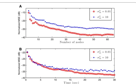
1 × 10⁻⁴ kg/m2. The total number of random realiza-tions used for simularealiza-tions is 100. The measurements are taken at every 0.5 s time-step starting from 0.5 s end-ing at 30 s. In the case of BLUE estimator, the received noise variance at the fusion center is assumed to be
σm2 =0.01, 10 m2.
Figure 3 shows the normalized mean squared error (MSE) and CRLB (in dB) with the increase in the number of nodes and samples. The normalized MSE and CRLB are obtained by dividing each with the diffusive field vol-ume. As one would expect, the estimation error decreases as more distributed nodes and samples are considered for estimation purpose. Since it is a 2D location estimation
problem, we need at least three nodes to determine the source location correctly. It is interesting to note that the estimation performance is slightly better than the CRLB in some cases. This is due to the fact that the ML esti-mator in this case is biased (suggested from simulation), and thus can outperform the CRLB by trading variance for bias. In this particular case, the continuous diffusive source can be localized with a resolution of less than 12 cm.
10 20 30 40 50 60 −50
−40 −30 −20 −10 0
Normalized MSE (dB)
0 5 10 15 20 25 30
−50 −40 −30 −20 −10 0
Normalized MSE (dB)
A
B
Figure 3Performance of MLE.Normalized MSE and CRLB of the MLE as function of(A)number of nodes, and(B)time samples.
A
B
model in (17). However, the performance of the BLUE estimator-based localization improves as the number of nodes and/or time samples increases. This is because for N,T → ∞, the complementary error function in (12) tends to be equal to 1, causing the linearization to have almost no effect on the approximation.
6.3 Moving diffusive source tracking
In this subsection, we analyze the performance of our pro-posed moving diffusive source tracking scheme. We use the same sensor network setup as described in Section 6.2. The initial source state vector is assumed to be Gaussian with meanμ =[0, 0, 0, 0]T and covariance matrix0 =
diag[0.01, 0.01, 0.01, 0.01]T. The intensity of the state process noise isσu2 = 0.1. The sampling time is assumed to beTs =0.5 s, and the total number of random realiza-tions used for simularealiza-tions is 50. The tracking is performed for 30 s and the number of particles in the PF isNp = 1, 000. The rest of the parameters is same as in Section 6.2. The performance measure is taken as the root mean squared error (RMSE) of the moving source position
esti-mate given by RMSEk = &
xs,k− ˆxs,k 2
+ys,k− ˆys,k 2
. The RMSE is compared with the square root of the PCRLB components of the position error, PCRLBk ≈
Ik−1 11+
I−k1
22.
Figures 5 and 6 show the tracking performances of the proposed tracking scheme using particle filter for grid-based and random node deployment strategies, respec-tively. It can be seen that the target trajectory can be tracked with better accuracy in Figure 6 compared to that in Figure 5. Figures 5B and 6B show the RMSEs on the tracking performances for the aforementioned two node deployment strategies respectively. The obtained RMSE with the random node deployment case is bet-ter and closer to the derived PCRLB than those of the grid-based node deployment case. This is because for a fixed node density, the expected nearest neighbor node distance (from the source) in case of random node deploy-ment is less than the inter-node spacing in grid-based node deployment, which in our case is 14.3 m. The ran-dom node deployment is specially suitable when there is no pre-designed infrastructure for sensor network and also when the diffusive field is hazardous for human deployment.
It is of interest also to investigate the performance of the proposed target tracking method when the sampling timeTsis varying. Figure 7 shows the effect of sampling time Ts on the tracking performances of the proposed moving diffusive source tracking scheme using grid-based node deployment strategy, keeping all the other param-eters same as mentioned before. As one would expect,
−14 −12 −10 −8 −6 −4 −2 0
−2 0 2 4 6
x−pos
y−pos
Actual Estimated
0 5 10 15 20 25 30
−30 −25 −20 −15 −10 −5 0
time (sec)
RMSE (dB)
RMSE PCRLB
A
B
Start End
−14 −12 −10 −8 −6 −4 −2 0 −2
0 2 4 6
x−pos
y−pos
0 5 10 15 20 25 30
−30 −25 −20 −15 −10 −5
time (sec)
RMSE (dB)
Actual Estimated
RMSE PCRLB
Start End
A
B
Figure 6Performance of the proposed tracking method with random sensor node deployment.(A)Actual and estimated trajectories of the moving diffusive source and(B)RMSE (dB) for random sensor node deployment.
−14 −12 −10 −8 −6 −4 −2 0
−2 0 2 4 6
x−pos
y−pos Actual trajectory
Estimated trajectory with T s=0.5s Estimated trajectory with T
s=1s
0 5 10 15 20 25 30
−25 −20 −15 −10 −5 0
time (sec)
RMSE (dB) RMSE with Ts=0.5s
PCRLB with Ts=0.5s RMSE with Ts=1s PCRLB with T
s=1s
Start End
A
B
the tracking performance decreases with the increase of sampling timeTs. This is because for higher values ofTs, the process noise will increase according to (23). Since we are also assuming that the movement of the diffu-sive source is almost linear between two succesdiffu-sive time instants, the lowerTswill result in better accuracy of the proposed tracking scheme.
7 Conclusion
In this paper, we obtained spatio-temporal distribution of the substance concentration by solving physical dif-fusion model for an underwater oil spill scenario which considers laminar water velocity as an external force. The obtained mathematical model was found to be capable of modeling satisfactorily the underlying physi-cal diffusion phenomenon. We proposed two paramet-ric estimation methods based on MLE and BLUE for determining static diffusive source location using wire-less sensor network. We also obtained the CRLB as theoretical performance bound for source localization. It was observed that though the MLE performs bet-ter than the BLUE-based diffusive source localization method, the latter shows satisfactory performance trend for large number of sensing nodes and time samples. We also proposed a particle filter-based target track-ing method for movtrack-ing diffusive source-emitttrack-ing sub-stance continuously into the dispersive medium. PCRLB corresponding to the moving diffusive source track-ing was obtained as a theoretical performance mea-sure and was compared with the simulation results. The effect of sampling time on the moving source tracking was also investigated. The performance of the proposed estimation and tracking methods are shown to be excellent using numerical simulations. In future research, we plan to combine our obtained analytical results with non-model-based numerical techniques to make them applicable for more realistic and complex scenarios.
Appendices Appendix 1
Derivation of spatio-temporal concentration in (9)
To derive and verify the spatio-temporal concentration distribution in (9), the Green’s functioncG(r,t)in (8) can be written ascG(r,t)=c1(r,t)+c2(r,t)+c3(r,t)+c4(r,t), where
c1(r,t)= 1
8{π κw(t−tI)}3/2 exp
−|r−r0−v(t−tI)|2 4κw(t−tI)
,
c2(r,t)= 1
8{π κw(t−tI)}3/2
exp
−|r−r−v(t−tI)|2 4κw(t−tI)
,
c3(r,t)= 1 4{π κw(t−tI)}3/2
exp
−{x−x0−vx(t−tI)}2
4κw(t−tI)
−{y−y0−vy(t−tI)}2 4κw(t−tI)
×
∞
n=1
exp
−(z−z0−2nL)2
4κw(t−tI)
, and
c4(r,t)= 1 4{π κw(t−tI)}3/2
exp
−{x−x0−vx(t−tI)}2
4κw(t−tI)
−{y−y0−vy(t−tI)}2
4κw(t−tI)
×
∞
n=1
exp
−(z+z0+2nL)2
4κw(t−tI)
.
Therefore, we can rewritec1(r,t)in (9) as
c1(r,t)=μ t
tI
c1(r,t−τ )dτ,= t
tI
μ
8{π κw(t−τ+tI)}3/2
×exp
−|r−r0−v(t−τ+tI)|2
4κw(t−τ+tI)
dτ,
= t−tI
0
μ (4π κwτ )3/2
exp
−|r−r0−vτ|2
4κwτ
dτ;
[performing change of variables],
(30)
To prove that (30) indeed translates into the expression given in (9), we will use the concept of first fundamen-tal theorem of calculus [41]. Sincec1(r,t)is a continuous real-valued function within the limits of the integral, the derivate of the expression given in (9) will be taken to obtain (30). Replacingγ = t−tIand assumingF(r,t) = c1(r,t)in (9), we have
F(r,γ )= μ
8π κw|r−r0|exp
(r−r0)·v
2κw exp
|r−r0||v|
2κw
×erfc
|r−r0|
2√κwγ + |v|
γ 4κw
+exp
−|r−r0||v|
2κw
×erfc |
r−r0|
2√κwγ − | v|
γ 4κw
.
Since dzderfc(z) = −√2
πexp(−z
2), we can obtain the
∂F(r,γ )
Similarly, we can also verify the expressions for c2(r,t) andc4(r,t). Therefore, the spatio-temporal concentration distributionc(r,t)given in (9) is valid.
Appendix 2 Proof of Theorem 1
We first show the proof for thexcoordinateθ0(1) = x0 and it can be easily followed to prove the consistency for the y and z coordinates without any loss of generality. Based on the technique in [30], we have to prove that
lim
∂x0 are continuous func-tions ofx0, by using Cauchy-Schwarz inequality, we can obtain Sbeing some positive real value. For practical considera-tion, assuming 0 ≤ |xj−x0|
can be written as
IfdN,T =N3T3>0 forN ≥1,T ≥1, then we can claim real numbers, we obtain the following from (15):
N to the diffusive source localization problem is consistent when the number of sensor nodes and time samples go to infinity.
Appendix 3 Proof of Theorem 2
To prove the asymptotic normality of the MLE, we define j,kyj,k|θ Below, we verify the necessary conditions mentioned in [42] for our obtained MLE to be asymptotically normal.
From practical point of view, there is no loss in gen-erality in assuming that θ0 ∈
◦
, where ◦ ⊂ is an open subset of . Also because the obtained MLE to source localization is consistent, it is also consistent even when θ0 ∈
is a continuous map-ping of θ, we can claim that ¨j,kyj,k|θ
is indeed uniformly continuous on θ in j and k [41]. Also, because ¨j,kyj,k|θ
: yj,k → R is a continuous
function of yj,k with yj,k being Lebesgue measurable
function, ¨j,kyj,k|θ
is also a measurable function of yj,k and condition N4 is satisfied. To satisfy N5,
exist and are bounded for all u,v. Hence, using the Cauchy-Schwarz inequality, all the leading principle minors of¯Iθ(inTheorem 2) can be shown to be positive. Thus, we can claim that I¯θ is also positive-definite and thereforeN7 is satisfied. BecauseE)ej,k* = σ positive finite number andN8 is satisfied.
To prove condition N9 since ¨j,k,u,vyj,k|θ
is a uni-formly continuous function of θ (shown in condition N4), for any > 0, there exists oneδ > 0 such that is a finite real number.
Therefore, the obtained MLE of the diffusive source location is asymptotically normal when the number of sensor nodes and time samples go to infinity.
Appendix 4 Proof of Theorem 3
Forp(s0)∼ N(μ0,0), the initial condition for the FIM
Since error is independent across space and time, using the concept from block matrix inversion, the information submatrix that provides the mean square error estimate of s1is given by
whereD1=E)−s1
−FTQ−1. Similarly, decomposing S2asS2=[sT0,s1T,sT2]T, the FIMI(S2)can be written as follows:
By extending the above procedure and decomposingSk+1=
sT0,sT1,. . .,skT+1T,ISk+1
can be obtained as
I(Sk+1)=
Similarly the only non-zero elements ofMk+1= −E
where the partial-derivative components are defined as follows:
∂ζj,k:k+1
Following the same approach as above, the elements of the matrixLk+1 ∈ R4×4k can easily be obtained at each time instant.
Abbreviations
BLUE: Best linear unbiased estimator; CRLB: Cramér-Rao lower bound; FC: Fusion center; FIM: Fisher information matrix; ML: Maximum-likelihood; MLE: Maximum-likelihood estimator; MSE: Mean squared error; PDF: Probability density function; PF: Particle filter; PCRLB: Posterior Cramér-Rao lower bound; SNR: Signal-to-noise-ratio; RMSE: Root mean squared error; WSN: Wireless sensor network.
Competing interests
Both authors declare that they have no competing interests.
Acknowledgements
This research was supported in part by the National Science foundation (NSF) under the grant CCF-0830545.
Received: 12 July 2012 Accepted: 18 May 2013 Published: 18 September 2013
References
1. JP Fitch, E Raber, DR Imbro, Technology challenges in responding to biological or chemical attacks in the civilian sector. Science.
302(5649), 1350–1354 (2003)
2. HT Banks, C Castillo-Chavez,Bioterrorism: Mathematical Modeling Applications in Homeland Security(Society for Industrial and Applied Mathematics, Philadelphia, 2003)
3. H Ishida, T Nakamoto, T Moriizumi, inInternational Conference on Solid State Sensors and Actuators. Remote sensing and localization of gas/odor source and distribution using mobile sensing system (Chicago, IL, 16–19 June 1997), pp. 559–562
4. A Nehorai, B Porat, E Paldi, Detection and localization of vapor-emitting sources. IEEE Trans. Signal Process.43, 243–253 (1995)
5. A Jeremic, A Nehorai, Design of chemical sensor arrays for monitoring disposal sites on the ocean floor. IEEE J. Oceanic Eng.23(4), 334–343 (1998)
6. RC Hughes, GC Osboum, JW Bartholomew, JL Rodriguez, inThe 8th International Conference on Solid-State Sensors and Actuators, and Eurosensors IX. Transducers ’95. The detection of mixtures of NOx’s with hydrogen using catalytic metal films on the Sandia robust sensor with pattern recognition (Stockholm, 25–29 June 1995), pp. 730–733 7. J Weimer, B Sinopoli, BH Krogh, inProceedings of the 30th IEEE Real-Time
Systems Symposium (RTSS). Multiple source detection and localization in advection-diffusion processes using wireless sensor networks (Philadelphia, 1–4 December 2009), pp. 333–342
9. M Ortner, A Nehorai, A Jeremic, Biochemical transport modeling and Bayesian source estimation in realistic environments. IEEE Trans. Signal Process.55(6), 2520–2532 (2007)
10. T Zhao, A Nehorai, Detecting and estimating biochemical dispersion of a moving source in a semi-infinite medium. IEEE Trans. Signal Process.
54(6), 2213–2225 (2006)
11. M Ortner, A Nehorai, A sequential detector for biochemical release in realistic environments. IEEE Trans. Signal Process.55(8), 4173–4182 (2007) 12. IF Akyildiz, W Su, Y Sankarasubramaniam, E Cayirci, Wireless sensor
networks: a survey. Comput. Netw.38(4), 393–422 (2002)
13. HR Trankler, O Kanoun, inProceedings of the 18th IEEE Instrumentation and Measurement Technology Conference (IMTC). Recent advances in sensor technology, vol. 1 (IEEE, New York, 2001), pp. 309–316
14. TK Hamrita, NP Kaluskar, KL Wolfe, in40th IAS Annual Meeting Industry, Industry Applications Conference. Advances in smart sensor technology, vol. 3 (IAS, Kowloon, 2005), pp. 2059–2062
15. CH Zhiyong, LY Pan, Z Zeng, inProceedings of the IEEE International Conference on Automation and Logistics Shenyang. A novel FPGA-based wireless vision sensor node (Shenyang, China, 5–7 August 2009), pp. 841–846
16. MS Lebold, B Murphy, D Boylan, K Reichard, inIEEE Aerospace Conference. Wireless technology study and the use of smart sensors for intelligent control and automation (Big Sky, MT, 5–12 March 2005), pp. 1–15 17. Micro-chemical sensors for in-situ monitoring and characterization of
volatile contaminants. (Sandia National Laboratories, 2005) http://www. sandia.gov/sensor/MainPage.htm. Accessed 1 September 2013 18. Cheaper chemical sensor. (MIT Technology Review) http://www.
technologyreview.com/tomarket/414073/cheaper-chemical-sensor/. Accessed 1 September 2013
19. J Chen, K Yao, R Hudson, Source localization and beamforming. IEEE Signal Process. Mag.19(2), 30–39 (2002)
20. P Stoica, J Li, Lecture notes - source localization from range-difference measurements. IEEE Signal Process. Mag.23(6), 63–66 (2006) 21. T Zhao, A Nehorai, Distributed sequential Bayesian estimation of a
diffusive source in wireless sensor networks. IEEE Trans. Signal Process.
55(4), 1511–1524 (2007)
22. H Zhang, JMF Moura, B Krogh, Dynamic field estimation using wireless sensor networks: tradeoffs between estimation error and communication cost. IEEE Trans. Signal Process.57(6), 2383–2395 (2009)
23. S Vijayakumaran, Y Levinbook, TF Wong, Maximum likelihood localization of a diffusive point source using binary observations. IEEE Trans. Signal Process.55(2), 665–675 (2007)
24. Y Lu, P Dragotti, M Vetterli, in49th Annual Allerton Conference on Communication, Control, and Computing. Localization of diffusive sources using spatiotemporal measurements (Monticello, IL, 28–30 September 2011), pp. 1072–1076
25. X Wang, S Wang, Collaborative signal processing for target tracking in distributed wireless sensor networks. J. Parallel and Distributed Comput.
67, 501–515 (2007)
26. H Ma, BW Ng, inProceedings of IEEE International Conference on Industrial Informatics. Collaborative data and information processing for target tracking in wireless sensor networks (Singapore, 16–18 August 2006), pp. 647–652
27. D Li, K Wong, YH Hu, A Sayeed, Detection, classification and tracking of targets in distributed sensor networks. IEEE Signal Process. Mag.
19(2), 17–29 (2002)
28. F Zhao, J Shin, J Reich, Information-driven dynamic sensor collaboration for target tracking. IEEE Signal Process. Mag.19(2), 61–72 (2002) 29. SS Ram, VV Veeravalli, inIEEE Global Telecommununications Conference
(GLOBECOM). Localization and intensity tracking of diffusing point sources using sensor networks (Washington, DC, 26–30 November 2007), pp. 3107–3111
30. HV Poor,An Introduction to Signal Detection and Estimation(Springer, New York, 1994)
31. WI Tam, D Hatzinakos, inIEEE International Conference on Communications ‘Towards the Knowledge Millenium’. An adaptive Gaussian sum algorithm for radar tracking, vol. 3 (Montreal, 8–12 June 1997), pp. 1351–1355 32. NJ Gordon, DJ Salmond, AM Smith, Novel approach to
non-linear/non-Gaussian Bayesian state estimation. IEEE Proc. F Radar and Signal Process.140, 107–113 (1993)
33. SM Kay,Fundamentals of Statistical Signal Processing: Estimation theory (Prentice Hall, Upper Saddle River, 1993)
34. P Tichavsky, CH Muravchik, A Nehorai, Posterior Cramer-Rao bounds for discrete-time nonlinear filtering. IEEE Trans. Signal Process.46, 1386–1396 (1998)
35. J Crank,The Mathematics of Diffusion(Oxford University Press, Oxford, 1975)
36. W Jost,Diffusion in Solids, Liquids, Gases(Academic Press Inc., New York, 1952)
37. D Duffy,Transform Methods for Solving Partial Differential Equations (Symbolic and Numeric Computation Series, Chapman & Hall/CRC, Boca Raton, 2004)
38. JC Lagarias, JA Reeds, MH Wright, PE Wright, Convergence properties of the Nelder-Mead simplex method in low dimensions. SIAM J. Optimization.9, 112–147 (1998)
39. AS Chhetri, D Morrell, A Papandreou-Suppappola, inIEEE Workshop on Statistical Signal Processing. Scheduling multiple sensors using particle filters in target tracking (St. Louis, MO, 28 September to 1 October 2003), pp. 549–552
40. P Djuric, J Kotecha, J Zhang, Y Huang, T Ghirmai, M Bugallo, J Miguez, Particle filtering. IEEE Signal Process. Mag.20, 19–38 (2003)
41. W Rudin,Principles of Mathematical Analysis(McGraw-Hill, New York, 1976) 42. B Hoadley, Asymptotic properties of maximum likelihood estimators for
the independent not identically distributed case. Ann. Math Stat.
42(6), 1977–1991 (1971)
doi:10.1186/1687-6180-2013-147
Cite this article as:Hakim and Jayaweera:Source localization and tracking in a dispersive medium using wireless sensor network.EURASIP Journal on Advances in Signal Processing20132013:147.
Submit your manuscript to a
journal and benefi t from:
7Convenient online submission
7Rigorous peer review
7Immediate publication on acceptance
7Open access: articles freely available online
7High visibility within the fi eld
7Retaining the copyright to your article
![Figure 2 Spatio-temporal concentration distribution. Concentration distribution in space (x-y-z coordinates) at times (A) t = 1 s and(B) t = 100 s with velocity vector v =[50, 50, 0] m/s (magnitude of concentration is proportional to the darkness).](https://thumb-us.123doks.com/thumbv2/123dok_us/902271.1108857/10.595.60.540.86.495/concentration-distribution-concentration-distribution-coordinates-magnitude-concentration-proportional.webp)