A DFT based approximate eigenvalue and singular value decomposition of polynomial matrices

R E S E A R C H

Open Access

A DFT-based approximate eigenvalue and

singular value decomposition of polynomial

matrices

Mahdi Tohidian

, Hamidreza Amindavar

and Ali M Reza

Abstract

In this article, we address the problem of singular value decomposition of polynomial matrices and eigenvalue decomposition of para-Hermitian matrices. Discrete Fourier transform enables us to propose a new algorithm based on uniform sampling of polynomial matrices in frequency domain. This formulation of polynomial matrix

decomposition allows for controlling spectral properties of the decomposition. We set up a nonlinear quadratic minimization for phase alignment of decomposition at each frequency sample, which leads to a compact order approximation of decomposed matrices. Compact order approximation of decomposed matrices makes it suitable in filterbank and multiple-input multiple-output (MIMO) precoding applications or any application dealing with realization of polynomial matrices as transfer function of MIMO systems. Numerical examples demonstrate the versatility of the proposed algorithm provided by relaxation of paraunitary constraint, and its configurability to select different properties.

1 Introduction

Polynomial matrices have been used for a long time for modeling and realization of input multiple-output (MIMO) systems in the context of control theory [1]. Nowadays, polynomial matrices have a wide spectrum of applications in MIMO communications [2-6], source separation [7], and broadband array processing [8]. They also have a dominant role in development of multirate filterbanks [9].

More recently, there have been much interest in poly-nomial matrix decomposition such as QR decomposition [10-12], eigenvalue decomposition (EVD) [13,14], and sin-gular value decomposition (SVD) [5,11]. Lambert [15] has utilized Discrete Fourier transform (DFT) domain to change the problem of polynomial EVD to pointwise EVD. Since EVD is obtained at each frequency separately, eigen-vectors are known at each frequency up to a scaling factor. Therefore, this method requires many frequency samples to avoid abrupt changes in adjacent eigenvectors.

*Correspondence: [email protected]

1Department of Electrical Engineering, Amirkabir University of Technology, P.O. Box 15914, Tehran, Iran

Full list of author information is available at the end of the article

Although, many methods of designing principle com-ponent filterbanks have been developed that are equiv-alent to EVD of pseudo circulant polynomial matrices [16,17], the next pioneering work on polynomial matrix EVD is presented by McWhirter et al. [13]. They use an extension of Jacobi algorithm known as SBR2 for EVD of para-Hermitian polynomial matrices which guar-antees exact paraunitarity of eigenvector matrix. Since final goal of SBR2 algorithm is to have strong decor-relation, the decomposition does not necessarily satisfy spectral majorization property. SBR2 algorithm has also been modified for QR decomposition and SVD [10,11].

Jacobi-type algorithms are not the only proposed meth-ods for polynomial matrix decomposition. Another itera-tive method for spectrally majorized EVD is presented in [14] which is based on the maximization of zeroth-order diagonal energy. Spectral majorization property of this algorithm is verified via simulation. Followed by the work of [6], a DFT-based approximation of polynomial SVD is also proposed in [18] which uses model order truncation by phase optimization.

In this article, we present polynomial EVD and SVD based on DFT formulation. It transforms the problem of polynomial matrix decomposition to the problem

of, pointwise in frequency, constant matrix decomposi-tion. At first it seems that applying inverse DFT on the decomposed matrices leads to polynomial EVD and SVD of the corresponding polynomial matrix. However, we will show later in this article that in order to have compact order decomposition, phase alignment of decomposed constant matrices in DFT domain results in polyno-mial matrices with considerably lower order. For this reason, a quadratic nonlinear minimization problem is set up to minimize the decomposition error for a given finite order constraint. Consequently, the required num-ber of frequency samples and computational complexity of decomposition reduce dramatically. The algorithm pro-vides compact order matrices as an approximation of polynomial matrix decomposition for an arbitrary poly-nomial order. This is suitable in MIMO communications and filterbank applications, where we deal with realiza-tion of MIMO linear time invariant systems. Moreover, formulation of polynomial EVD and SVD in DFT domain enables us to select the property of decomposition. We show that if eigenvalues (singular values) intersect at some frequencies in frequency domain, smooth decomposition, and spectrally majorized decomposition are distinct. The proposed algorithm is able to reach to either of these properties.

The remainder of this article is organized as fol-lows. The relation between polynomial matrix decom-position and DFT matrix decomdecom-position is formulated in Section 2. In Section 3, two important spectral prop-erties of decomposition, namely spectral majorization and smooth decomposition, are provided using appro-priate arrangement of singular values (eigenvalues) and corresponding singular vectors (eigenvectors). The equal-ity of polynomial matrix and dft matrix decomposed matrices decompositions are guaranteed via the finite duration constraint, which is investigated in Section 4. The finite duration constraint imposes the phase angles of singular vector (eigenvector) to minimize a nonlin-ear quadratic function. A solution for this problem is proposed in Section 5. Section 6 presents the results of some computer simulations which are considered to demonstrate performance of the proposed decomposition algorithm.

1.1 Notation

Some notational conventions are as follows: constant val-ues, vectors, and matrices are in regular character lower case, lower case over-arrow, and upper case, respectively. Coefficients of polynomial (scalar, vector, and matrix) are with indeterminate variablenin the square brackets. Any polynomial (scalar, vector, and matrix) is distinguished by bold character and indeterminate variable z in the parenthesis and its DFT by bold character and indetermi-nate variablekin the brackets.

2 Problem formulation

Denote ap×qpolynomial matrixA(z)such that each ele-ment ofA(z)is a polynomial. Equivalently, we can indicate this type of matrix by coefficient matrixA[n],

A(z)=

The polynomial matrix multiplication of ap×qmatrix A(z)and aq×tmatrixB(z)is defined as

C(z) = A(z)B(z)

cij(z) = q_k=1aik(z)bkj(z).

We can obtain the coefficient matrix of product by matrix convolution ofA[n] andB[n], that is defined as

C[n] = A[n]∗B[n]

cij[n]= q

k=1aik[n]∗bkj[n]

where∗denotes the linear convolution operator. Denote para-conjugate of a polynomial matrix as

˜

A(z)=AT_∗(z−1)=

Nmax

Nmin

AH[n]zn.

in which,∗as a subscript denotes the complex conjugate of coefficients in the polynomial matrixA(z).

A matrix is said to be para-Hermitian ifA˜(z)=A(z)or equivalentlyA[n]=AH[−n]. We call a polynomial matrix paraunitary if U˜(z)U(z) = I, whereIis aq×qidentity matrix.

Thin EVD of ap×ppara-Hermitian polynomial matrix A(z)is of the form

A(z)=U(z)(z)U˜(z), (2)

and thin SVD of ap×qarbitrary polynomial matrix is of the form,

A(z)=U(z)(z)V˜(z) (3)

whereU(z)andV(z)arep×randq×rparaunitary matri-ces, respectively.(z)and(z)representr×rdiagonal matrices whereris the rank ofA(z).

We can equivalently write EVD of a para-Hermitian matrix and SVD of a polynomial matrix in coefficient matrix form

A[n]=U[n]∗[n]∗UH[−n] (4)

A[n]=U[n]∗[n]∗VH[−n] (5)

In general, EVD and SVD of a finite-order polynomial matrix are not finite order. As an example, suppose EVD of para-Hermitian polynomial matrix

Eigenvalues and eigenvectors of the polynomial matrix in (6) are neither of finite order nor rational

(z)=

The same results can be found for polynomial QR decomposition in [12].

We mainly explain the proposed algorithm for polyno-mial SVD, yet wherever it seems necessary we explain the result for both decomposition.

The decomposition in (3) can also be approximated by samples of discrete-time Fourier transform, yields a decomposition off the form

A[k]=U[k][k]VH[k] , k=0, 1,. . .,K−1. (7)

Such a decomposition can be obtained by taking theK -point DFT of coefficient matrixA[n],

A[k]=A(z)|_z=wk

DFT formulation plays an important role in decomposi-tion of polynomial matrices because it replaces the prob-lem of polynomial SVD that involves many protracted steps withK conventional SVD that are pointwise in fre-quency. It also enables us to control spectral properties of the decomposition. However, it causes two inherent drawbacks:

1. Regardless of what is the trajectory of polynomial singular values in frequency domain, conventional SVD order singular values irrespectively of the ordering in neighboring frequency samples.

2. In frequency domain, samples of polynomial singular vectors are known up to a scalar complex

exponential by using the SVD at each frequency sample, which yields to discontinuous variation between neighboring frequency samples.

The first issue is directly dealt with the spectral proper-ties of the decomposition. In Section 3, we would explain why arranging singular values in decreasing order yields to approximate spectral majorization, while smooth decom-position requires rearrangement of singular values and their corresponding singular vectors.

For the second issue, suppose conventional SVD of an arbitrary constant matrix A. If the pairu and vare the left and right singular vectors corresponding to a non-zero singular value, for an arbitrary scalar phase angleθ, the pairejθ_uandejθ_{vare also left and right singular vectors}

corresponding to the same singular value. Although this non-uniqueness is trivial in conventional SVD, it plays a crucial role in polynomial SVD. When we perform SVD at each frequency of DFT matrix as in (7), these non-uniquenesses in phase exist at each frequency regardless of other frequency samples. Moreover, in many applications, specially those which are related to MIMO precoding, we can relax constraints of the problem by letting singular values to be complex (see applications of polynomial SVD in [4,18])

⎧

Given this situation, singular values have not all their conventional meaning. For instance, the greatest singu-lar value is conventionally 2-norm of the corresponding matrix, which is not true for complex singular values. The process of compensating singular vectors for these phases is what we callphase alignmentand is developed in Section 4.

Based on what was mentioned above, Algorithm 1 gives the descriptive pseudo code for DFT-based SVD. Modifi-cations of the algorithm for EVD of para-Hermitian matri-ces are straightforward. If at each frequency sample all

singular values are in decreasing order, REARRANGE

function (which is described in Algorithm 2) is only required for smooth decomposition, otherwise for spec-tral majorization, no further arrangement is required. For the phase alignment, first we need to compute phase angles which is indicated in the algorithm by DOGLEG

function and is described in Algorithm 3.

3 Spectral majorized decomposition versus smooth decomposition

Two of the most appealing decomposition properties are

Algorithm 1Approximate SVD

U[n] ,[n] ,V[n]←ASVD(A[n])

for k=0, 1,· · ·,K−1

Compute A[k] from (8):

A[k]=Nmax

NminA[n]w

kn K Decompose A[k] from (7):

U[k] ,[k] ,V[k]←SVD(A[k])

end(for)

If smooth decomposition is required use Algorithm 2:

U[k] ,[k] ,V[k]←REARRANGEU[k] ,[k] ,V[k]

for i=1, 2,· · ·,r

Compute phase angles using Algorithm 3:

θ_iu[k] ,θ_iv[k]←DOGLEGu_i[k] ,v_i[k]

for k=0, 1,. . .,K−1

Phase alignment using (9) or (10) end(for)

end(for)

for n=0, 1,. . .,M−1

Compute decomposed polynomial matrices: U[n]←K_k=0U[k]W−kn

V[n]←K_k=0V[k]W−kn

[n]← Diagonal elements of UH_{[−n]∗A[n]∗V[n]} end(for)

time, hence we should choose which one we are willing to use as our main objective.

In many filterbank applications which are dealt with principle components filterbank, spectral majoriza-tion and strong decorrelamajoriza-tion are both required [16]. Since smooth decomposition leads to more compact decomposition, in cases that the only objective is strong decorrelation, exploiting smooth decomposition is reasonable. The DFT-based approach of polyno-mial matrix decomposition is capable of decomposing a matrix with either of these properties with small modification.

Polynomial EVD of a para-Hermitian matrix is said to have spectral majorization property if [13,16]

λ1(ejω)≥λ2(ejω)≥ · · · ≥λr(ejω), ∀ω.

Note that, eigenvalues corresponding to para-Hermitian matrices are real in all frequencies.

We can extend the definition to the polynomial SVD, replacing singular values with eigenvalues in the defini-tion, we have

σ1(ejω)≥σ2(ejω)≥ · · · ≥σr(ejω), ∀ω.

If we let singular values to be complex, we can replace absolute value of singular values in the definition.

A polynomial matrix have no discontinuity in frequency domain, hence we modify definition of smooth decompo-sition presented in [19] to fit with our problem and avoid unnecessary discussions.

Polynomial EVD (SVD) of a matrix is said to possess smooth decomposition if eigenvectors (singular vectors) have no discontinuity in frequency domain, that is

_ddωuil(e

jω_{)<∞, ∀ω and} i=1, 2,. . .,r

l=1, 2,. . .,p, (11)

whereuilis thelth element ofui.

If eigenvalues (singular values) of a polynomial matrix intersect at some frequencies, the spectral majorization and smooth decomposition are not simultaneously realiz-able. As an example, supposeA(z)is a polynomial matrix with u1(z) and u2(z) are eigenvectors corresponding to distinct eigenvalues λ1(z) and λ2(z), respectively. Lets assumeu1(ejω)andu2(ejω) have no discontinuity in fre-quency domain, andλ1(ejω)andλ2(ejω)intersect at some frequencies. Denote

λ₁(ejω)=

λ₁(ejω) λ₁(ejω)≥λ₂(ejω)

λ2(ejω) λ1(ejω) <λ2(ejω) ,

λ₂(ejω)=

λ2(ejω) λ1(ejω)≥λ2(ejω)

Algorithm 2Rearrangement for smooth decomposition which implies that they are not smooth anymore. In this situation, although λ₁(ejω), λ₂(ejω), u₁(ejω), and u₂(ejω) are not even analytic, we can approximate them with finite order polynomials.

If a decomposition has spectral majorization, its eigen-values (singular eigen-values) are of decreasing order in all frequencies. Therefore, they are in decreasing order in any arbitrary frequency sample set, including DFT frequen-cies. Obviously the converse is only approximately true. Hence, for polynomial EVD to possess spectral majoriza-tion approximately, it suffices to arrange sampled eigen-values (singular eigen-values) of (7) in decreasing order. Since we only justify spectral majorization at DFT frequency sam-ples, the resulting EVD (SVD) may possess the property only approximately. Similar results can be seen in [14,20].

To have smooth singular vectors, we propose an algo-rithm based on inner product of consecutive frequency samples of singular vectors. We can accumulate smooth-ing requirement in (11) for allrelements as

_ddωui(e

jω₎

<∞, ∀ω and i=1, 2,. . .,r. (14) LetBbe the upper bound of norm of derivative and{·} be the real value of a complex value.

For an arbitraryωwe have

can be made to be as close to unity as desired by makingωsufficiently small. In our problemui(ejω)

is sampled uniformly withω = 2_Kπ. Since EVD is per-formed at each frequency sample independently, ui[k]

and ui[k+ 1] are not necessarily two consecutive

fre-quency samples of a smooth eigenvector. Therefore, we should rearrange eigenvalues and eigenvectors to yield smooth decomposition. This can be done for each sam-ple of eigenvector ui[k] by seeking for the eigenvector

of successor sample uj[k + 1] with the most value of

computation of {cu_ij[k]} is not possible before phase alignment. Due to (15), for sufficiently smallω, two con-secutive samples of a smooth singular vector can be as close as desired and we can approximate

cu_ij[k] the intersection of eigenvalues, consecutive eigenvectors which are sorted by conventional EVD in decreasing order, are from the same smooth eigenvector and so

|cu₁₁[k]|and|cu₂₂[k]|are near unity. However, ifk−1 and

kare two frequency sample before and after the intersec-tion, respectively, due to decreasing order of eigenvalues, smoothed eigenvectors are swapped after intersection. Therefore,|cu₁₁[k]|and|cu₂₂[k]|are some values near zero, instead|cu₁₂[k]|and|cu₂₁[k]|are near unity.

Algorithm 2 describes a simple rearrangement proce-dure to track eigenvectors (singular vectors) for smooth decomposition.

4 Finite duration constraint

Phase alignment is critical to have compact order decom-position. Another aspect of this fact is revealed in the coefficient’s domain perspective of (7). In this domain, the multiplication is replaced by circular convolution

A[((n))K]= U[((n))K][((n))K]VH[((−n))K] = U[((n))K][((n))K]VH[((−n))K]

(16)

Polynomial SVD corresponds to linear convolution in the coefficients domain, however the decomposition obtained from DFT corresponds to circular convolution. Recalling from discrete-time signal processing, it is well known that we can equivalently utilize circular convolution instead of linear convolution if convoluted signals are zero-padded adequately. That is, forx1[n] andx2[ 2] are two signals with the length ofN1andN2, respectively, apply zero padding such that zero padded signals have the lengthN1+N2−1 [21]. Hence, if the lastM−1 coefficients ofU[n],[n], and

V[n], are zero, the following results are hold:

A[((n))K]=U[((n))K][((n))K]VH[((−n))K]⇒A[n]=U[n]∗[n]∗VH[−n] ,

U[((n))K]UH[((−n))K]=δ[((n))K]I⇒U[n]∗UH[−n]=δ[n]I,

V[((n))_K]VH[((−n))_K]=δ[((n))_K]I⇒V[n]∗VH[−n]=δ[n]I.

(17)

Therefore, the problem is to obtain the phase set {θ_i[k]} and correcting the singular vectors using (9). The phase set{θ_i[k]}should be such that the resulting coefficients satisfy (17).

Without loss of generality, letU[n] andV[n] be causal, i.e.,U[n]= V[n]= 0 forn < 0.U[n] andV[n] (which are supposed to be of lengthM) should be multi-sequence zero-padded at least with(M−1)zeros.

U[n]= 1 these conditions are satisfied, circular convolution can be used instead of linear convolution.

Since the available matrix of singular vectors at each frequency isU[k], inserting (9) in (18) for each singular vector separately leads to

pact form we can express these(K−M)-folded equations in matrix form

For polynomial EVD, Equation (20) is enough, however, for polynomial SVD we have two options. To approximate SVD with approximately positive singular values, we must

augmentFM(u_i) andfM(u_i) with similar defined matrix

An additional degree of freedom is obtained by letting singular values to be complex. However, an straightfor-ward solution which yield to singular values and singular vectors of orderMis complicated. Instead, we impose the finite duration constraint only two singular vectors

FM(u_i)x(θiv)= −fM(u_i)

FM(v_i)x(θiv)= −fM(v_i)

i=1, 2,. . .,r. (22)

IfK≥2M−1, then the lastM−1 coefficients of resulting polynomial vectors are zero. Therefore, according to (17), U(z)andV(z)are paraunitary. On the other hand, ifK ≥ ing singular values, we have two options, we can either set

M. Another option which yields to more accurate results is by calculatingU˜(z)A(z)V(z)and replacing off-diagonal elements with zero.

Next, we provide a minimization approach to determine the unknown set{θi[k]}.

5 Gradient descent solution

In general, there may exist no phase vectorθwhich sat-isfies (20). Even when there exists a phase vector that satisfies the finite duration constraint, the solution is not straightforward. For these reasons, we can view (20) as a minimization problem [6]. We use energy of the highest order coefficients (the coefficients that we equate to zero in (18)) as the objective to the minimization problem

J(θi)=FM(u_i)x(θiu)+ fM(u_i)

2

, i=1, 2,. . .,r.

(23)

An alternative minimization technique as a solution for this phase optimization problem is proposed in [6], which we describe it in this section.

Throughout this section, we focus on solving θ_i = arg minJ(θ_i)as a least square solution for a single singular vectorui[k], so we drop the subscript “i” from the

quan-tityθi and useF andf, instead ofFM(u_i) andfM(u_i)to

simplify the notation. The objectiveJ(θ ) is intentionally presented as a function ofθto emphasize the fact that our problem is classified as an unconstrained optimization.

We exploit the trusted region strategy for the prob-lem (23). By utilizing the information about the gradient vector and Hessian matrix in each step, trusted region strategy constructs a model functionmkwhich have a

sim-ilar behavior close to the current pointθ(k). The model

mk is usually defined as the second-order Taylor series

expansion (or its approximation) ofJ(θ+ ϕ) aroundθ, that is

mk(ϕ) =J(θ ) + ϕT∇J(θ ) + ϕT∇2J(θ )ϕ,

where∇J(θ ) and∇2J(θ ) are the gradient vector and the Hessian matrix corresponding toJ(θ ), respectively. The modelm_k is designed to be a good approximation ofJ(θ ) near the current point and is not trustworthy on regions far from the current point. Consequently, the restriction in minimization ofmkon a region aroundθ(k)is crucial,

that is

whereRis the trusted region radius.

The decision about shrinking of the trusted region is determined by comparing the actual reduction inobjective

function and predicted reduction. Given a stepϕ, the ratio

ρ= J(θ ) −J(θ+ ϕ)

mk(0)−mk(ϕ)

(25)

is used as a criterion to indicate if the trusted region is small enough.

Among methods which approximate the solution of the constrained minimization (24) dogleg procedure is the only one which leads to analytical approximation. It also promises to achieve at least as much reduction inmkas is

possible by Cauchy point (the minimizer ofmk along the

steepest descent direction−∇J(θ ), subject to the trusted region) [22]. However, this procedure requires Hessian matrix (or an approximation of it) to be positive definite.

5.1 Hessian matrix modification

The gradient vector and Hessian matrix corresponding to

J(θ ) are as follows

In general, Hessian matrix in (26) does not promise to be always positive definite. Therefore, we should modify Hessian matrix to yield a positive definite approximation.

We provide a simple modification which brings some desirable features by omitting the second term from the Hessian matrix and diagonal loading to guarantee positive definiteness

H(θ ) ≈2X(θ)FHFX(θ)H+αI. (27)

The term 2X(θ)FHFX(θ)H is positive semi-definite and in many situations, it is much more significant than the second term of Hessian matrix in (26). Hence, with diagonal loadingαI (Iis with conformable size andα is very small), the modified Hessian matrix guarantees (27) to be positive definite and provides the desired properties in contrast to use the exact Hessian matrix.

5.2 Dogleg method

Dogleg method starts with the unconstrained minimiza-tion of (24)

φh= −H−1g (28)

When the trusted region radius is so large thatφH ≤

Algorithm 3Trusted region dogleg algorithm

Evaluate ρ_i from (25) if ρi< 1₄

The dogleg method approximates this trajectory by a path consisting of two line segments. The first line seg-ment starts from the origin to the unconstrained mini-mized point along the steepest descent direction

φg= − g

T_g

gT_Hgg. (29)

The second line segment starts fromφgtoφh. These two line segments form an approximate trajectory which its intersection with the sphereφ = Ris the approximate solution of (24) whenφh>R.

5.3 Alternating minimization

Another solution of (23) is provided by converting the problem of multivariate minimization to a sequence of single-variate minimization problem via alternating min-imization [6]. In each iteration, a series of single-variate minimization is performed, while other parameters are held unchanged. Each Iteration consists of K −1 steps,

which at each step one parameterθ[k] is updated. Sup-pose we are at stepkof ith iteration. At this stepk−1 first parameters were updated in the current iteration, and

K−k−2 last parameters were updated from the previ-ous iteration. These parameters are held fixed, whileθ[k] is minimized at the current step,

θ_i[k]=arg min

θ[k]

J(θi[1],...,θi[k−1],θ[k],θi−1[k+1],...,θi−1[K−1]).

(30)

The cost function is guaranteed to be non-incremental at each step; however, this method is also converges to a local minima which highly depend on the initial guess of the algorithm. For solving (30) it is suffices to make the

kth element of gradient vector in (26) equal to zero. Sup-pose the calculation are performed for phase alignment of

Fortunately, Equation (31) has a closed form solution

θi[k]=

∠ti[k]

∠ti[k]+π. (32)

However, only the second case of (32) has positive second partial deviation. Therefore, the global minima of (30) is

θi[k]=∠ti[k]+π.

5.4 Initial guess

All algorithms of unconstrained minimization require to be supplied by a starting point, which we denoted byθ0. To avoid getting stuck in local minima, we should select a good initial guess. This can be accomplished by min-imizing a different but similar cost function denoted by

J(θ )

J(θ ) =x(θi)−F†f

2

in which†represents pseudo inverse. SolvingJ(θ ) yields to a simple initial guess

θ0=∠F†f. (33)

we start with the initial guess of (33) and a trusted region radius upper bound R¯. Then we continue the trusted region minimization procedure as described in this section.

6 Simulation results

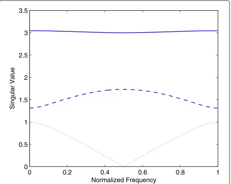
In this section, we present some examples to demonstrate the performance of the proposed algorithm. For the first example, our algorithm is applied to a polynomial matrix example from [11]

Frequency behavior of singular values can be seen in Figure 1. There is no intersection of singular values, so the setup of the algorithm either for spectral majorization or frequency smoothness leads to identical decomposition.

For having approximately positive singular values, we use (21). Define the average energy of highest order coef-ficients for the pair of polynomial singular vectorsuiand

viasEui,v = J(θi)/(K−M)(we expect energy of highest

order coefficients to be zero or at least minimized). A plot ofEi versus iteration for each pair of singular vectors is depicted in Figure 2. The decomposition length isM=9 (order is 8) and we useK = 2M+(Nmax−Nmin) = 20 number of DFT points.

As it is seen, the use of dogleg method with approximate Hessian matrix leads to a fast convergence in contrast with using alternative minimization and Cauchy-point (which is always selected along the gradient direction). Of course we should consider that due to matrix inversion, computa-tional complexity of Dogleg method isO(K3)while com-putational complexity of alternative minimization and Cauchy point isO(K2).

Figure 1Singular values versus frequency.

The final value of average highest order coefficient for three pair of singular vectors are 5.54 × 10−5_{, 3.5 ×} 10−3_{, and 0.43, respectively. The first singular vector} sat-isfies finite duration constraint almost exactly. The second singular vector fairly satisfies this constraint. However, highest order coefficients of last singular vector, pos-sess considerable amount of energy, that seems to cause decomposition error.

Denote the relative error of the decomposition as

EA=

A(z)−U(z)(z)V˜(z)

F A(z)_F

in which ·F is the extension of Frobenius norm for

polynomial matrices and is defined by

A(z)F =

n

A[n]2_F.

Since in our optimization procedure we only seek for finite duration approximation, U(z) and V(z) are only approximately paraunitary. Therefore, we also define rela-tive error of paraunitarity as

EU =

U˜(z)U(z)−I

F

r .

An upper bound forEU can be obtained as

EU≤2

which means as average energy onK−Mhighest order goes to zero,EUdiminishes.

The relative error of this decomposition isEA=1.18× 10−2while the error ofU(z)andV(z)areEU =3.3×10−2 and EV = 3.08 × 10−2, respectively. The paraunitar-ity error is relatively high in contrast with decomposition error. This is due to the difference between the first two singular values and the last singular value.

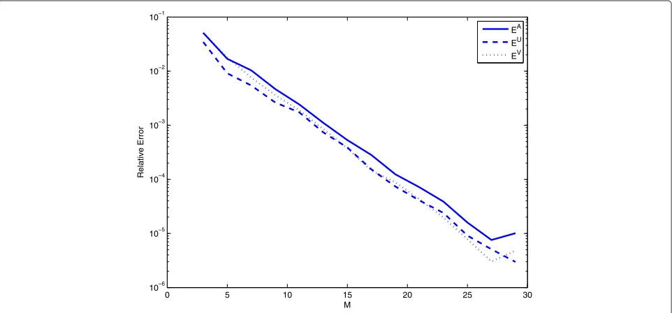
A plot of relative errors EA_{, E}U_{, and E}V _{for various}

amount of Mis shown in Figure 3. The number of fre-quency samples is fixed atK =2M+2(Nmax−Nmin).

The number of frequency samples K is an optional

0 10 20 30 40 50 60 70 80 90 100 10−5

100 105

Iteration Number

E1

0 10 20 30 40 50 60 70 80 90 100 10−5

100 105

Iteration Number

E2

0 10 20 30 40 50 60 70 80 90 100 100

Iteration Number

E3

Figure 2Average highest order coefficients energyEiversus iteration number for a decomposition with approximately positive singular

values.Dotted line: Cauchy points. Dashed line: Alternative minimization. Solid Line: proposed algorithm.

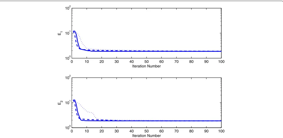
Now, lets relax the problem by allowing singular values to be complex and using (22). A plot ofE_iuandE_ivversus iteration for each pair of singular vectors is depicted in Figure 5. The decomposition length isM= 9 (order is 8) and we useK = 2M+(Nmax−Nmin) = 20 number of DFT points.

Again Dogleg method converges very rapidly while alternative minimization and Cauchy point converge slowly. The final value of average energy for three left singular vectors are 1.23×10−10, 9.7×10−4, and 10−3,

0 5 10 15 20 25 30 35 40 45 10−3

10−2 10−1 100 101

M

Relative Error

EA EU EV

Figure 3Relative error versusMfor a decomposition with approximately positive singular values.K=2M=2.

respectively. This is while these values for right singu-lar vectors are 1.12 × 10−10, 1.4 × 10−3, and 8.7−4, respectively.

Note that the average energy of highest order coeffi-cients for the third pair of singular vectors alleviate mean-ingfully. Figure 1 shows that the third singular value goes to zero and then returns to positive values. If we constrain singular values to be positive, a phase jump ofπ radian, is imposed to one of third singular vectors near the fre-quency which singular vector goes to zero. However, by

30 40 50 60 70 80 90 100 10−3

10−2 10−1 100

K

Relative Error

EA EU EV

0 20 40 60 80 100 10−20

100 1020

Iteration Number

E

u 1

0 20 40 60 80 100 10−10

100 1010

Iteration Number

E

v 1

0 20 40 60 80 100 10−5

100 105

Iteration Number

E

u 2

0 20 40 60 80 100 10−4

10−2 100

Iteration Number

E

v 2

0 20 40 60 80 100 10−5

100 105

Iteration Number

E

u 3

0 20 40 60 80 100 10−5

100 105

Iteration Number

E^v_3

Figure 5Average highest order coefficients energyEiversus iteration number for a decomposition with complex singular values.Dotted

line: Cauchy points. Dashed line: Alternative minimization. Solid Line: proposed algorithm.

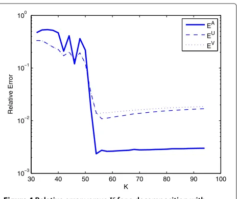
letting singular values to be complex, the zero crossing occur which requires no discontinuity of singular vectors. The relative error of this decomposition isEA = 4.9× 10−3_{while the error ofU(z)andV(z)areE}U _=2.5×10−3 andEV _{= 3.5×10}−3_{, respectively. In contrast with} con-straining singular values to be positive, having complex singular values decrease decomposition and paraunitarity error significantly.

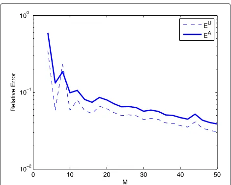
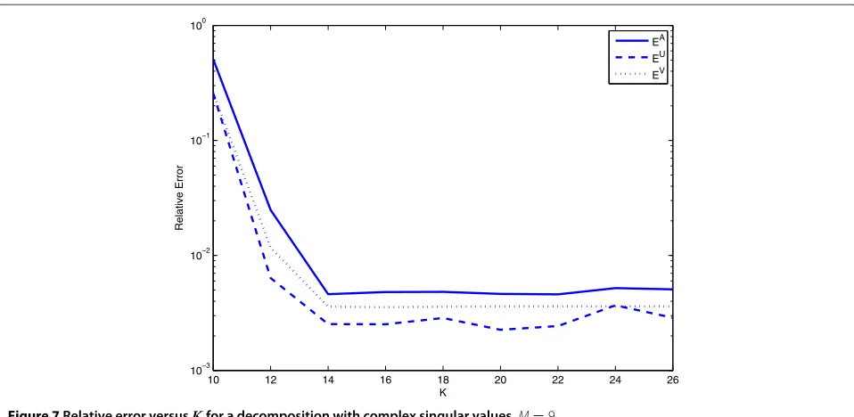
Plots of relative errors EA, EU, and EV for various

amount of M and K are shown in Figures 6 and 7,

respectively. Letting singular values be complex causes

significant reduction of all relative errors. As it was men-tioned, Figure 7 shows that increasingKfrom 2M+Nmax−

Nmin−1 causes no improvement in relative errors while it makes additional computational burden.

McWhirter and coauthors [11] have reported the rel-ative error of decomposition. Provided that paraunitary matricesU(z)andV(z)are of order 33, the relative error of their algorithm is 0.0469. This is while our algorithm only requires paraunitary matrices of order 3 for relative error of 0.035 with positive singular values and relative error of 2.45×10−6with complex singular values. In addition,

0 5 10 15 20 25 30

10−6 10−5 10−4 10−3 10−2 10−1

M

Relative Error

EA

EU

EV

10 12 14 16 18 20 22 24 26 10−3

10−2 10−1 100

K

Relative Error

EA

EU

EV

Figure 7Relative error versusKfor a decomposition with complex singular values.M=9.

in the new approach, exploiting paraunitary matrices of order 33, the relative error is 0.0032 with positive singular values and 4.7×10−6with complex singular values.

This large difference is not caused by iteration num-bers because we compare results while all algorithms relatively converges, and with continuation of iterations trivial improvement are obtained. The main reason lies on different constraints of the solution presented in [11] in contrast to our proposed method. While they impose paraunitary constraint onU˜(z)A(z)V(z)to yield a diago-nalized(z), we impose the finite duration constraint and obtain approximation of U(z) and V(z) with fair fitting to the decomposed matrices at each frequency samples. Therefore, we can consider this method as a finite dura-tion polynomial regression of matrices which is obtained by uniformly samplingU(z)andV(z)on the unit circle in

z-plane.

As a second example, consider EVD of the following para-Hermitian matrix

A(z)=

.5z2+3+.5z−2 −.5z2+.5z−2

.5z2−.5z−2 −.5z2+1−.5z−2

The exact smooth EVD of this matrix is of finite order

U(z)= 1 2

1+z−1 1−z−1

1−z−1 _1+z−1

, (35)

(z)=

z1+2+z−1 0

0 −z1+2−z−1

.

Frequency behavior of eigenvalues can be seen in Figure 8. Since eigenvalues intersect at two frequencies,

smooth decomposition and spectrally majorized decom-position result two distinct solutions.

To perform smooth decomposition, we need to track and rearrange eigenvectors to avoid any discontinuity using Algorithm 2. The resulting |cu_ij[k]| are shown in Figure 9 fork = 0, 1,. . .,K−1. Using these|cu_ij[k]|the Algorithm 2 swap first and second eigenvalues and eigen-vectors for k = 12 : 32 which results in continuity of eigenvalues and eigenvectors.

Now that all eigenvalues and eigenvectors are rear-ranged in DFT domain, it’s time for phase alignment of

0 0.2 0.4 0.6 0.8 1

0 0.5 1 1.5 2 2.5 3 3.5 4

Normalized Frequency

Eigenvalue

0 5 10 15 20 25 30 35 40 45 0

0.1 0.2 0.3 0.4 0.5 0.6 0.7 0.8 0.9 1

k

Figure 9Rearrangement of eigenvalues and eigenvectors.K=42. Dashed Line:cu₁₂[k] andcu₂₁[k]. Solid Line:cu₁₁[k] andcu₂₂[k].

eigenvectors. A plot ofEiversus iteration forM =3 and

smooth decomposition is depicted in Figure 10. It is pre-dictable that dogleg algorithm converges rapidly while the alternative minimization and Cauchy point has a long way to converge.

Since the energy of highest order coefficients of eigen-vectors are trifling, using the proposed method for smooth decomposition results in very high accuracy, as

seem in the figures. Relative error of smooth decomposi-tion versusMis shown in Figure 11.

While using frequency smooth EVD of (35) leads to rel-ative error below 10−5forM ≥ 3 with a few number of iterations, Spectrally majorized EVD requires a lot more polynomial order to reach a reasonable relative error.

Unlike smooth decomposition which requires rear-rangement of eigenvalues and eigenvectors, spectral

0 10 20 30 40 50 60 70 80 90 100 10−30

10−20 10−10 100 1010

Iteration Number E1

0 10 20 30 40 50 60 70 80 90 100 10−30

10−20 10−10 100 1010

Iteration Number E2

Figure 10Eiversus iteration number corresponding to smooth decomposition.Dotted line: Cauchy points. Dashed line: Alternative

0 5 10 15 10−15

10−10 10−5 100

M

Relative Erro

r

EA EU

Figure 11Relative error of smooth decomposition versusM.

majorization requires only to sort eigenvalues at each frequency sample in decreasing order. Most of con-ventional EVD algorithm sort eigenvalues in decreasing order, which we should only align eigenvector phases

using 3. A plot of Ei versus iteration for M = 20

and spectrally majorized decomposition is depicted in Figure 12.

Due to an abrupt change in eigenvectors at the intersec-tion frequency of eigenvalues, increasing the decomposi-tion order leads to a slow decay of relative error. Figure 13 shows the relative error as a function ofM.

To see the difference between smooth and spectrally majorized decomposition results, eigenvalues of spec-trally majorized decomposition is shown in Figure 14, which is comparable with Figure 8 which corresponds to eigenvalues of smooth decomposition. Therefore, a low order polynomial is required using smooth decomposi-tion and much higher polynomial order for spectrally majorized decomposition. Even withM=20 the decom-position have relatively high error.

7 Conclusion

An algorithm for polynomial EVD and SVD based on DFT formulation has been presented. One of the advan-tages of the DFT formulation is that it enables us to control properties of decomposition. Among these prop-erties, we introduce how to setup the decomposition to achieve spectrally majorization and frequency smooth-ness. We have shown, if singular values (eigenvalues) intersect at some frequency, then simultaneous achieve-ment of spectral majorization and smooth decomposition is not possible. In this situation, setting up the decom-position to possess spectral majorization requires con-siderably higher order polynomial decomposition and more computational complexity. Highest order polyno-mial coefficients of singular vectors (eigenvectors) are utilized as square error to obtain a compact decompo-sition based on phase alignment of frequency samples. The algorithm has the flexibility to compute a decom-position with approximately positive singular values, and

0 10 20 30 40 50 60 70 80 90 100 100

101 102

Iteration Number E1

0 10 20 30 40 50 60 70 80 90 100 100

101 102

Iteration Number E2

Figure 12Eiversus iteration number corresponding to spectrally majorized decomposition.Dotted line: Cauchy points. Dashed line:

0 10 20 30 40 50

Figure 13Relative error of spectrally majorized decomposition versusM.

a more relaxed decomposition with complex singular values. A solution for this nonlinear quadratic problem is proposed via Newton’s method. Since we apply an approximate Hessian matrix to assist the Newton opti-mization, a fast convergence is achieved. The algorithm capability to control the order of polynomial elements of decomposed matrices and to select properties of decom-position, make the proposed method as a good choice for filterbank and MIMO precoding applications. Finally, performance of the proposed algorithm under different conditions is demonstrated via simulations. Simulation results reveal superior decomposition accuracy in con-trast with coefficient domain algorithms due to relaxation of paraunitarity.

Figure 14Eigenvalues of spectrally majorized decomposition versus frequency.M=20.

Competing interests

The authors declare that they have no competing interests.

Author details

1_{Department of Electrical Engineering, Amirkabir University of Technology,} P.O. Box 15914, Tehran, Iran.2_{Electrical Engineering and Computer Science,} University of Wisconsin-Milwaukee, P.O. Box 784, Milwaukee, WI 53201–0784, USA.

Received: 1 March 2012 Accepted: 15 March 2013 Published: 30 April 2013

References

1. T Kailath,Linear Systems. ( Prentice Hall, Englewood Cliffs, NJ, 1980) 2. J Tugnait, B. Huang, Multistep linear predictors-based blind identification

and equalization of multiple-input multiple-output channels. IEEE Trans. Signal Process.48(1), 569–571 (2000)

3. R Fischer, Sorted spectral factorization of matrix polynomials in MIMO communications. IEEE Trans. Commun.53(6), 945–951 (2005) 4. H Zamiri-Jafarian, M Rajabzadeh, inIEEE Vehicular Technology Conference,

VTC Spring 2008. A polynomial matrix SVD approach for time domain

broadband beamforming in MIMO-OFDM systems, (2008), pp. 802–806 5. R Brandt, Polynomial matrix decompositions: evaluation of algorithms

with an application to wideband MIMO communications (2010). Master of Science in Engineering Physics Thesis, Uppsala University, Uppsala, Sweden,

6. D Palomar, M Lagunas, A Pascual, A Neira, inInternational Symposium on Signal Processing and Its Applications, ISSPA. Practical implementation of jointly designed transmit-receive space-time IIR filters, (2001), pp. 521–524 7. R Lambert, A Bell, inProceedings of the International Conference on

Acoustics, Speech, and Signal Processing. Blind separation of multiple speakers in a multipath environment, (1997), pp. 423–426 8. S Redif, J McWhirter, P Baxter, T Cooper, inOCEANS 2006. Robust

broadband adaptive beamforming via polynomial eigenvalues, (2006), pp. 1–6

9. P Vaidyanathan,Multirate Systems and, Filterbanks, 4th edn. (Prentice Hall, Englewood Cliffs, 1993)

10. J Foster, J McWhirter, J Chamber, inProceedings of the International

Conference on Acoustics, Speech, and Signal Processing. A novel algorithm

for calculating the QR decomposition for a polynomial matrix, (2009), pp. 3177–3180

11. J Foster, J Mcwhirter, M Davies, J Chambers, An algorithm for calculating the QR and singular value decompositions of polynomial matrices. IEEE Trans. Signal Process.58(3), 1263–1274 (2010)

12. D Cescato, H Bolcskei, QR decomposition of Laurent polynomial matrices sampled on the unit circle. IEEE Trans. Inf. Theory.56(9),

4754–4761 (2010)

13. J Mcwhirter, P Baxter, T Cooper, S Redif, An EVD algorithm for para-Hermitian polynomial matrices. IEEE Trans. Signal Process.55(5), 2158–2169 (2007)

14. A Tkacenko, inProceedings of the International Conference on Acoustics,

Speech, and Signal Processing. Approximate eigenvalue decomposition of

para-Hermitian systems through successive FIR paraunitary transformations ((Dallas, Texas, USA, 2010), pp. 4074–4077 15. R Lambert, Multichannel blind deconvolution: FIR matrix algebra and

separation of multipath mixtures (1996). PhD Thesis, University of Southern California, Los Angeles

16. P Vaidyanathan, Theory of optimal orthonormal subband coders. IEEE Trans. Signal Process.46(4), 1528–1543 (1998)

17. A Tkacenko, P Vaidyanathan, On the Spectral Factor Ambiguity of FIR Energy Compaction Filter Banks. IEEE Trans. Signal Process.54(1), 146–160 (2006)

18. R Brandt, M Bengtsson, inInternational Symposium on Personal, Indoor,

and Mobile Radio Communication. Wideband MIMO channel

diagonalization in the time domain, (2011), pp. 1958–1962 19. L Dieci, T Eirola, On smooth decomposition of matrices. SIAM J. Matrix

20. S Redif, J McWhirter, S Weiss, Design of FIR paraunitary filter banks for subband coding using a polynomial eigenvalue decomposition. IEEE Trans. Signal Process.59(11), 5253–5264 (2011)

21. A Oppenheim, R Schafer, J Buck,Discrete-Time Signal Processing, 2nd edn. (Prentice Hall, Englewood Cliffs, 1999)

22. J Nocedal, S Wright,Numerical Optimization. (Springer, New York, 1999)

doi:10.1186/1687-6180-2013-93

Cite this article as:Tohidianet al.:A DFT-based approximate eigenvalue and singular value decomposition of polynomial matrices.EURASIP Journal on Advances in Signal Processing20132013:93.

Submit your manuscript to a

journal and benefi t from:

7Convenient online submission 7Rigorous peer review

7Immediate publication on acceptance 7Open access: articles freely available online 7High visibility within the fi eld

7Retaining the copyright to your article