Prediction of Fast Fading Parameters by Resolving the Interference Pattern
Tugay Eyce¨oz and Alexandra Duel-Hallen
North Carolina State University
Dept. of Electrical & Computer Engineering
Box 7914, Raleigh, NC 27606-7914
[email protected], [email protected]
Hans Hallen
North Carolina State University
Physics Department
Box 8202, Raleigh, NC 27695-8202
Hans [email protected]
Abstract
In this paper, we investigated a new deterministic ap-proach to the estimation and prediction of the fading chan-nel by exploiting the physical nature of the flat fading signal. Since the direct signal and the reflected signals form an in-terference pattern, the received signal is given by a sum of several scattered components. These are distinguished by their Doppler shifts at the mobile. The slowly varying pa-rameters associated with these components are determined and tracked, and the composite fading signal is predicted. This approach will potentially result in the ability to an-ticipate and avoid "deep fades" which severely limit the performance of wireless communications systems and will aid in the development of low power mobile radio systems.
1. Introduction
The mobile radio channel places fundamental limitations on the performance of wireless communication systems [1, 2, 3]. The transmission path between the transmitter and the receiver can be severely obstructed by terrain con-figuration and the man-made environment. These result in multiple paths between the source and the receiver, caus-ing significant variations in the amplitude and the phase of the received signal, known as fading. For simplicity, we concentrate on the flat fading channel. Consider a low-pass complex model of the received signal:
r (t)=c(t)s(t)+n(t) (1)
wherec(t)is the flat fading coefficient (multiplicative),s(t)
is the transmitted signal, andn(t)is additive white Gaussian
noise (AWGN).
Let the transmitted signal be s(t) = P
k b
k
g (t;k T),
whereb
k is the data sequence,
g (t)is the transmitter pulse
This research was supported by NSF grants 9410227 and NCR-9726033.
shape, and T is the symbol delay. At the output of the
matched filter and sampler, the discrete-time system model is given by
y k
=c k
b k
+z
k (2)
where c
k is the fading signal
c(t) sampled at the symbol
rate, andz
kis the discrete AWGN process. It is well known
thatc(t)andc
kcan be modeled as complex Gaussian random
processes with Rayleigh distributed amplitudes and uniform phases [1]. The expressions for the autocorrelation function and the power spectral density of the flat fading signal are also widely used in practice [4].
Several adaptive channel estimation methods have been developed by using this statistical description to estimate rapidly varying fading coefficients (e.g. [5, 6, 7, 8]). For example, the minimum mean square error (MMSE) estimate using the Kalman filter is usually found by constructing a Gauss-Markov model of the fading. In this model, the mean square error is given by the variance of the excitation noise. This error grows as the Doppler shift increases and limits the performance of the detector. Furthermore, the bit error rate (BER) approaches the saturation level (error floor) as the signal-to-noise ratio (SNR) increases.
Although the estimation error causes performance degra-dation, it is not the most serious limiting factor in commu-nication over fading channels. The greatest BER loss and the associated high power requirements result from "deep fades" in the fading signal. Therefore, it is desirable to predict deep fades, and, in general, fading variations and compensate for the expected power loss at the transmitter. Therefore, we address the deterministic prediction of the variations inc
k. By prediction we imply estimating an
en-tire future block of coefficientsc
k based on the observation
of future channel coefficients and does not introduce signifi-cant complexity increase relative to present communication techniques for fading channels.
2. Fading Channel Model
From the point of view of the mobile, the fading coeffi-cient at the receiver is given by a sum of N Doppler shifted signals [4]
c(t)= N X
n=1 A
n e
j2 f n
t+ n
(3)
where (for then th
scatterer)A
nis the amplitude, f
nis the
Doppler frequency, and
n is the phase. Moreover, the
Doppler frequency is given by
f n
=f c
( v
c )cos
n (4)
wheref
c is the carrier frequency,
vis the speed of mobile,
c is the speed of light, and
nis the incident angle
rela-tive to the mobile’s direction. Due to multiple scatterers, the fading signal varies rapidly for large vehicle speeds and undergoes "deep fades" [1, 3]. The complex Gaussian distri-bution of the fading signal (the Rayleigh fading) is derived based on the assumption that the scattered signals are dis-tributed uniformly around the mobile, and that there is a continuum of scatterers [4]. Although the exact derivation of the Rayleigh fading distribution requires this assumption, it has been demonstrated that the Rayleigh fading signal can be closely approximated by a relatively small number num-ber of scatterers. For example, in the popular deterministic Jakes model, as few as nine scatterers can be used to model Rayleigh fading characteristics [4]. Physical evidence sug-gest that the actual number of significant scattered signals is modest. All significant scatterers must have an amplitude similar to that of the most powerful signal, otherwise their interference effects will be negligible. Such signals will re-sult from specular (mirror-like) scattering from the ground, water, buildings or perhaps vehicles [3, 9, 10]. Trees and vegetation tends to absorb the signal so they will not be important in this analysis [9, 10, 11]. Since the specular reflection occurs close to a specific geometry and scatter-ing efficiencies are small enough (>10 dB loss/scattering
[9, 12]) that multiple scattering effects are greatly reduced, only a few scatterers are expected, as confirmed by obser-vations [13]. The assumption of small number of scatterers was also made in promising work on fading channel estima-tion presented in [14, 15].
We predict the fading signalc
k (2) by decomposing it
in terms of the N scattered components. If the parameters
A n,
f n, and
nin (3) for each of the scatterers were known
and remained constant, the signal could be predicted indef-initely. In practice, they vary slowly and are not known a
priori. Since we consider short term fading, the propaga-tion characteristics will not change significantly during any given block, and we can safely assume these parameters are approximately constant or change very slowly for the duration of the data block.
These slow variations in the parameters associated with scattered waveforms can also be explained by viewing the received signal from the frame of reference of the ground rather than mobile. In this frame of reference, the direct sig-nal and the reflected sigsig-nals from the transmitter combine to form an interference pattern. The mobile drives through this interference pattern. For the time interval under consid-eration, it can be assumed that it is moving at approximately constant speed and direction through this interference
pat-tern. As a result, the parameters A
n, f
n, and
n do not
change significantly. Therefore, it should be possible to measure and track the variations in the parameters.
3. Spectral Estimation and Linear Prediction
To predict the fading signals (2-3), we employ spectral estimation followed by linear prediction and interpolation.
Estimation of the power spectral density of discretely sampled deterministic and stochastic processes is usually based on procedures employing the Discrete Fourier Trans-form (DFT) [16]. Although this technique for spectral es-timation is computationally efficient, there are some per-formance limitations of this approach. The most important limitation is that of frequency resolution. The frequency resolution ( ∆f = f
s
=N ) of the N-point DFT algorithm,
wheref
sis the sampling frequency, limits the accuracy of
estimated parameters. These performance limitations cause problems especially when analyzing short data records.
Many alternative Spectral Estimation Techniques have been proposed within the last three decades in an attempt to alleviate the inherent limitations of the DFT technique [16, 17, 18]. We explore the Maximum Entropy Method (MEM) for the prediction of the fast fading signal. This method is also known as the All-poles Model or the Autoregressive (AR) Model and is widely used for spectral estimation. The reason why we chose this technique is that the MEM has very nice advantage of fitting sharp spectral features as we have in our fading channel due to scatterers (3). Furthermore, MEM is closely tied to Linear Prediction (LP) which we use to predict future channel coefficients. Using MEM, the frequency response of the channel is modeled as:
H(z)=
1
1;
P p j=1
d j
z j
: (5)
This model is obtained based on a block of samples of the
fading process. Note that the samples have to be taken
−1 −0.5 0 0.5 1 −1
−0.8 −0.6 −0.4 −0.2 0 0.2 0.4 0.6 0.8 1
Real part
Imaginary part
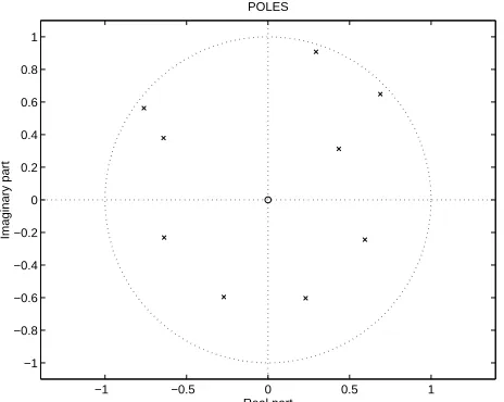
POLES
Figure 1. Pole-zero locations of the frequency response of the channel for three scatterers,
f d
=100Hz
Doppler frequency,f
d. Moreover, the accuracy of the model
depends on the number of samples in the given block. The
d
j coefficients are calculated from the poles of the power
spectral density.
The d
j coefficients in (5) are also the linear prediction
coefficients. The estimates of the future samples of the
fading channel can be determined as:
ˆ
c n
= p X
j=1 d
j c
n;j (6)
Thus, ˆc
n is a linear combination of the values of c
n over
the intervaln;p n;1]. Since actual channel coefficients
are not available beyond the observation interval, earlier sampling estimates, ˆc
n;j, can be used instead of the actual
valuesc
n;jin (6) to form future estimates ˆ c n.
Note that the channel sampling rate utilized for LP is much lower than the symbol rate, 1=T. Therefore, to predict
the fading coefficients,c
k (2), associated with transmitted
symbols, interpolation is employed as discussed in the next section.
4. Simulation Results
Numerical results illustrate performance characteristics of the proposed technique. In the examples, we assume that the maximum Doppler frequency is 100 Hz, and the data rate is 24 Ksps. We sample the channel at the rate of 240 Hz. Thus, there are 100 data points between adjacent sampling points. To determine the observations of the fading coefficients,c
k, at the sampling points, one can send training
0 5 10 15 20 25 30 35 40 45 50 0
0.2 0.4 0.6 0.8 1 1.2 1.4 1.6 1.8
Time −−> (in units of samples)
Amplitude
Figure 2. Actual ( — ) and estimated ( ... ) fading channel envelopes for 3 scatterers,
f d
=100Hz
symbolsb
kat the channel sampling rate of 240 Hz (see (2)).
This overhead affects the throughput only by 1%.
In order to give a better insight into the performance of this technique, we will first demonstrate the case of three scatterers (N =3 in (3)). In Figure 1, the pole-zero plot
of the frequency response of the channel found by MEM is illustrated. Note that the three poles corresponding to the three oscillators are placed very close to the unit cir-cle. The angles of these poles correspond to the oscillator
frequencies. With the sampling frequency, f
s
= 240 Hz,
these three Doppler frequencies correspond to 100 50 and 30 Hz. The plot of the envelope due to these scatterers is drawn in Figure 2. The channel is observed for the first 25 samples. Then, by employing MEM and Linear Predic-tion, the future values of the channel envelope are estimated and plotted using dotted lines for the last 25 samples in the figure. The estimates agree with actual values and we can detect when the channel will enter deep fades in the future. The same experiment is repeated in the presence of additive white Gaussian noise and the result is plotted in Figure 3. Note that the predicted values still follow very closely the actual channel envelope which is plotted in solid lines.
We also performed simulations for a greater number of scatterers. In Figures 4 and 5, the original Jakes channel model with nine oscillators (scatterers) is examined [4]. In Figure 4, the pole-zero plot of the frequency response of the Jakes channel model with a maximum Doppler frequency,
f d
= 100 Hz, is illustrated. As the number of oscillators
0 5 10 15 20 25 30 35 40 45 50 0
0.2 0.4 0.6 0.8 1 1.2 1.4 1.6 1.8
Time −−> (in units of samples)
Amplitude
Figure 3. Actual ( — ) and estimated ( ... ) fading channel envelopes for 3 scatterers in
the presence of AWGN, SNR=20dB
samples. We plotted the predicted channel envelope in dot-ted lines and the actual channel envelope in solid lines after the observation interval in Figure 5. It can be seen that the predicted values still follow very closely the actual channel envelope. However, later in the prediction, the accuracy de-creases because of the cumulative effect of the LP error. This error is due to the fact that earlier estimates rather than actual fading values are used in predicting future samples. We are currently addressing this problem by combining adaptive tracking at the receiver with prediction and power control at the transmitter.
Since the sampling rate for the fading channel is much lower than the data rate, we perform interpolation between predicted channel coefficients to get better resolution. In this interpolation process, four consecutively predicted channel coefficients are interpolated by a Raised Cosine (RC) filter to generate estimates of fading coefficients, ˆc
k, between two
middle predicted samples at the data rate [19]. The interpo-lation result and the actual channel coefficients are shown in Figure 6. The solid line represents the actual channel coeffi-cients,c
k, at the data rate. Two points, represented by , are
the estimated channel parameters. By using these points ( as well as one previous and one next estimate), we perform the interpolation at the data rate. These interpolated estimates,
ˆ
c
k are shown with dashed line in the figure. We prefer
in-terpolation to oversampling of the fading channel to obtain the fading coefficients at the data rate. If oversampling is employed, MEM will require a larger number of poles and consequently the complexity will increase.
−1 −0.5 0 0.5 1
−1 −0.8 −0.6 −0.4 −0.2 0 0.2 0.4 0.6 0.8 1
Real part
Imaginary part
Figure 4. Pole-zero locations of the frequency
response of the Jakes channel model, f
d =
100Hz
5. Future Work
We are currently investigating applications of the fading prediction method described in this paper to communica-tion system design. Feedback of received samples to the transmitter and subsequent fading prediction and compen-sation in the transmitter for the received signal power is studied. Note that the proposed method is not meant to replace adaptive channel estimation required for coherent detection. Instead, prediction will result in more reliable tracking of the received signal.
The capability to predict fading coefficients will reduce the power requirements of wireless communications sys-tems and increase the system performance. In particular, it would be possible to avoid transmission during deep fades or to utilize diversity techniques (e.g., use space diversity or hop to another non-fading frequency during the deep fade) [1, 3]. In addition, more efficient modulation and coding techniques are envisioned.
150 155 160 165 170 175 180 185 190 195 200 0
0.5 1 1.5 2 2.5
Time −−> (in units of samples)
Amplitude
Figure 5. Actual ( — ) and estimated ( ... ) fad-ing channel envelopes for the Jakes channel
model,f
d
=100Hz
References
[1] J. G. Proakis, Digital Communications, McGraw-Hill, New York, 1995.
[2] S. Stein, "Fading Channel Issues in System Engineering",
IEEE Transactions on Selected Areas in Communications,
5(2):68–89, February 1987.
[3] T. S. Rappaport, Wireless Communications, Prentice Hall, NJ, 1996.
[4] W. C. Jakes, Microwave Mobile Communications, John Wiley and Sons, New York, 1974.
[5] J. Lin, J. G. Proakis, F. Ling, and H. Lev-Ari, "Optimal Tracking of Time-Varying Channels: A Frequency Domain Approach for Known and New Algorithms", IEEE
Transac-tions on Selected Areas in CommunicaTransac-tions, 13(1):141–154,
Jan. 1995.
[6] R. Haeb and H. Mayr, "A Systematic Approach to Carrier Recovery and Detection of Digitally Phase Modulated Signals on Fading Channels", IEEE Transactions on Communications, 37(7):748–754, July 1989
[7] Z. Zvonar and M. Stanjovic, "Performance of Antenna Di-versity Multiuser Receivers in CDMA Channels with Imper-fect Channel Estimation", Wireless Personal Communications
Journal, Kluwer, 91–110, July 1996
[8] H. Y. Wu and A. Duel-Hallen, "Performance Comparison of Multiuser Detectors with Channel Estimation for Flat Raleigh Fading CDMA Channels", Special Issue on Interference in
Mobile Wireless Systems, Wireless Personal Communications Journal, Kluwer, in press
[9] A. Seville, U. Yilmaz, P. G. V. Charriere, N. Powel, and K. H. Craig, "Building Scatter and Vegetation Attenuation Mea-surements at 38 GHz", Proceedings of the 9th International
Conference on Antennas and Propagation, Eindhoven, the
Netherlands, 46–50, 1995
0 10 20 30 40 50 60 70 80 90 100 1.3
1.32 1.34 1.36 1.38 1.4 1.42 1.44 1.46 1.48 1.5
Time −−> (in unit of data samples)
Amplitude
Figure 6. (—): actual channel coefficients,c
k;
(;;;): interpolated channel estimates,cˆ
k
[10] T. J. Schmugge and T. J. Jackson, "A Dielectric Model of the Vegetative Effects on the Microwave Emission from Soils",
IEEE Transactions on Geoscience and Remote Sensing, 30(4):
757–760, 1992
[11] I. J. Dilworth and B . L’Ebraly, "Propagation Effects due to Foliage and Building Scatter at Millimeter Wavelengths",
Proceedings of the 9th International Conference on Antennas and Propagation, Eindhoven, the Netherlands, 51–53, 1995
[12] M. S. Ding and M. O. Al-Nuaimi, "Prediction of Scatter Coefficient of Buildings at Microwave Frequencies in Site Shielding", Proceedings of the 9th International Conference
on Antennas and Propagation, Eindhoven, the Netherlands,
42–45, 1995
[13] P. A. Mathews and B. Mohebbi, "Direction of Arrival and Building Scatter at UHF", Proceedings of 7th International
Conference on Antennas and Propagation, York, U.K., 147–
150, 1991
[14] M. K. Tsatsanis and G. B. Giannakis "Modeling and Equal-ization of Rapidly Fading Channels", Inter. Journal of
Adap-tive Control and Signal Processing, 10, 179–176, April 1996
[15] M. K. Tsatsanis and G. B. Giannakis "Equalization of Rapidly Fading Channels: Self-Recovering Methods", IEEE
Transac-tions on CommunicaTransac-tions, 44(5), 619–630, May 1996
[16] J. G. Proakis, D. G. Manolakis, Digital Signal Processing, Prentice Hall, NJ, 1996.
[17] M. H. Hayes, Statistical DSP and Modeling, John Wiley and Sons, 1996.
[18] S. M. Kay and S. L. Marple "Spectrum Analysis–A Modern Perspective", Proceedings of the IEEE, 69(11), 1380–1419, Nov. 1981