Modeling, Control and Power Sharing Methods for Distribution Systems Driven by Solid-State Transformers: A Nonlinear Dynamical Approach.

ABSTRACT

AFIAT MILANI, ALIREZA. Modeling, Control and Power Sharing Methods for Distribution Systems Driven by Solid-State Transformers: A Nonlinear Dynamical Approach. (Under the direction of Dr. Iqbal Husain and Dr. Aranya Chakrabortty.)

Intrusion of new intermittent generation sources such as wind and solar generators with associated power electronic converters, and highly stochastic loads such as plug-in electric vehicles in the distribution-end results in some technical challenges in the conventional power grid. One of the major challenges of this intrusion is the increase in the system node voltages when power generated by the renewable resources flows back to the grid. This regenerative power flow results in instability issues in the system. To minimize these problems, the Future Renewable Electric Energy Delivery and Management (FREEDM) system is proposed recently which consists of an energy router, i.e., the solid-state transformer (SST). SST is a controllable transformer with communication and intelligent control layers integrated with it that provides power and energy management, voltage and power factor control and low voltage and low frequency ride-through functionality. Another key feature that distinguishes the SST from a traditional transformer is its ability to decouple and buffer medium-voltage distribution grids from the low-voltage feeder sections where distributed renewable energy resources (DRER), distributed energy storage devices (DESD) and local loads are connected.

two power sharing methods are discussed which can be used to maintain the feasibility of the system in case there is a change in the load of one of the SSTs. In these methods, the other SSTs in the network help the SST in need by appropriately tuning their references.

In order to keep the system operational, aside from maintaining its feasibility, the operating point also needs to be stable. Based on the derived dynamic model, a globally asymptotically stabilizing controller for a multi-SST based FREEDM system using Lyapunov stability theory is proposed. The designed controller is centralized; however, by proper selection of controller gains, it can be simplified to be implemented in either a sparse or decentralized way. The performance of the controller under several load conditions and incorrect references in controller gains is studied.

Modeling, Control and Power Sharing Methods for Distribution Systems Driven by Solid-State Transformers: A Nonlinear Dynamical Approach

by

Alireza Afiat Milani

A dissertation submitted to the Graduate Faculty of North Carolina State University

in partial fulfillment of the requirements for the degree of

Doctor of Philosophy

Electrical Engineering

Raleigh, North Carolina 2018

APPROVED BY:

_______________________________ _______________________________

Dr. Iqbal Husain Dr. Aranya Chakrabortty Committee Co-Chair Committee Co-Chair

_______________________________ _______________________________

DEDICATION

BIOGRAPHY

ACKNOWLEDGMENTS

I would like to express my deepest gratitude to my advisors Dr. Iqbal Husain and Dr. Aranya Chakrabortty for their sincere guidance, advice and support to pursue my Ph.D. I feel blessed to have Dr. Husain, an outstanding scholar and a great mentor as my advisor, who taught me to conduct research in a fundamental way that results in a contribution with a meaningful impact. I am also very grateful to have Dr. Chakrabortty as my advisor. The completion of this research was not possible without his scientific advice and guidance. I would also like to extend my gratitude to my other Ph.D. committee members, Dr. Srdjan Lukic and Dr. Andre Mazzoleni for their valuable suggestions and feedbacks to improve my dissertation. I also thank Dr. Rafael Cisneros Montoya for his guidance during the last year of my PhD.

I would also like to thank all the faculty and staff at the NSF FREEDM systems center for providing tremendous support and encouragement. A special thanks goes to Ms. Karen Autry for her kindness and love. I would also like to thank Dr. Md Tanvir Arafat Khan for being a great friend and knowledgeable colleague in our FREEDM system modeling and control research project.

TABLE OF CONTENTS

LIST OF TABLES ... vii

LIST OF FIGURES ... viii

Chapter 1: Introduction ... 1

1.1 Research Background ... 1

1.2 Research Motivation ... 4

1.3 Contribution ... 6

1.4 Dissertation Outline ... 7

Chapter 2: Dynamic Modeling of a Solid-state Transformer Based Power Distribution System... 10

2.1 Introduction ... 10

2.2 Solid-state Transformer Dynamic Model ... 11

2.2.1 Front-end Rectifier ... 12

2.2.2 Dual-active Bridge Converter ... 17

2.2.3 Voltage Source Inverter ... 19

2.2.4 Overall SST Model ... 21

2.2.5 DC and AC Microgrids ... 21

2.3 Multi-SST FREEDM Dynamic Model ... 22

2.4 Case Studies and Simulation Results ... 23

2.5 Conclusion ... 28

Chapter 3: Feasibility Analysis of the FREEDM System... 29

3.1 Introduction ... 29

3.2 Single SST Feasibility Analysis... 30

3.2.1 Feasibility Analysis of Rectifier ... 32

3.2.2 Feasibility Analysis of DAB ... 36

3.2.3 Feasibility Analysis of Inverter ... 38

3.3 Expansion of Feasibility Region ... 39

3.4 Equilibrium Analysis with Multiple SSTs ... 43

3.5 Power Flow Analysis in Presence of Changes in System Load... 44

3.6 Case Studies and Simulation Results ... 50

3.7 Conclusion ... 53

Chapter 4: Controller Design for a Multi-SST FREEDM Distribution System ... 54

4.1 Introduction ... 54

4.2 SST-based Distribution Network Dynamic Model ... 55

4.3 Motivating Example... 58

4.4 Controller Design ... 60

4.4.1 Decentralized Controller Design ... 68

4.5 System Operation in Presence of Incorrect References in the Controller ... 69

4.5.1 Feasibility Analysis of the Closed-Loop System ... 70

4.6 FREEDM System Control in Absence of DESD Systems ... 71

4.6.1 Single SST FREEDM System ... 72

4.6.2 Multi-SST FREEDM System ... 73

4.7 Case Studies and Simulation Results ... 74

4.8 Conclusion ... 86

Chapter 5: FREEDM System in the Islanded Mode of Operation ... 87

5.1 Introduction ... 87

5.2 FREEDM System Dynamic Model in the Islanded mode ... 88

5.3 FREEDM System Feasibility Analysis in the Islanded mode ... 90

5.4 FREEDM System Stability Analysis in the Islanded mode ... 93

5.5 Case Studies and Simulation Results ... 94

5.6 Conclusion ... 97

Chapter 6: Summary and Future Work ... 98

6.1 Summary ... 98

6.2 Future Work ... 100

LIST OF TABLES

Table 3.1 Positive and negative power bounds of rectifier ... 41

Table 3.2 Power sharing test system load data ... 50

Table 4.1 Test system data ... 75

Table 4.2 Test system current references ... 76

LIST OF FIGURES

Figure 2.1 Solid-state transformer circuit model ... 12

Figure 2.2 Front-end rectifier circuit ... 13

Figure 2.3 Rectifier nested PI control scheme ... 16

Figure 2.4 Dual-active bridge circuit ... 18

Figure 2.5 DAB PI control scheme ... 18

Figure 2.6 Voltage source inverter circuit ... 19

Figure 2.7 Inverter PI control scheme ... 20

Figure 2.8 Single SST FREEDM system ... 22

Figure 2.9 Multi SST FREEDM system ... 23

Figure 2.10 SST dynamic performance under microgrid current variation ... 24

Figure 2.11 SST input current under microgrid current variation ... 25

Figure 2.12 SST input current dynamics under microgrid current variation ... 25

Figure 2.13 SST dynamic performance under load variation ... 26

Figure 2.14 SST dynamic performance under grid variation ... 27

Figure 2.15 SST input current under grid variation ... 27

Figure 2.16 SST dynamic performance under changes in other SSTs ... 28

Figure 3.1 Rectifier feasibility circles for 𝑃𝑟𝑒𝑐 = 50 𝑘𝑊 ... 36

Figure 3.2 Rectifier feasibility zone for power flow ... 42

Figure 3.3 Rectifier feasibility region expansion ... 42

Figure 3.4 Feasibility region in multi-SST distribution systems ... 45

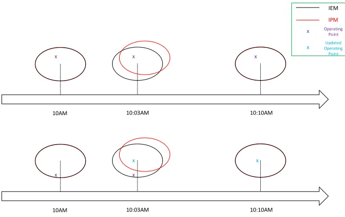
Figure 3.5 Control interaction between IEM and IPM ... 47

Figure 3.7 Input voltage of each SST by applying power sharing with

constant input current method ... 51

Figure 3.8 Input current of each SST by applying power sharing with constant input current method ... 51

Figure 3.9 Net power of each SST by applying power sharing with constant node voltage method ... 52

Figure 3.10 Input voltage of each SST by applying power sharing with constant node voltage method ... 52

Figure 3.11 Input current of each SST by applying power sharing with constant node voltage method ... 52

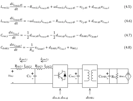
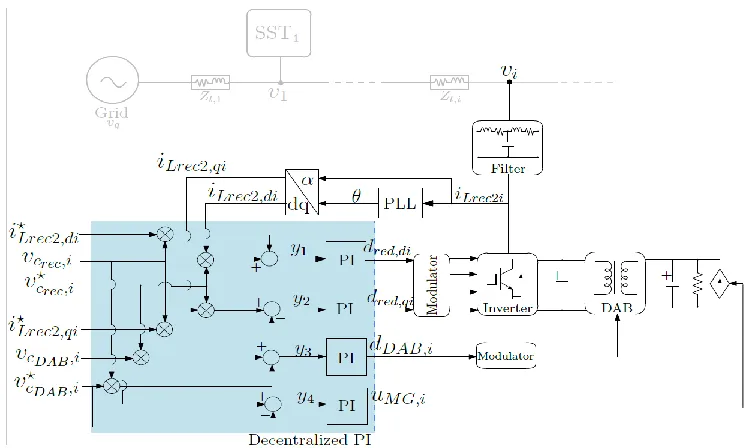
Figure 4.1 Schematic representation of 𝑆𝑆𝑇_𝑖 of FREEDM system ... 57

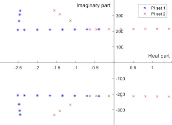
Figure 4.2 Stability diagram for a given single SST FREEDM system using nested PI controller ... 59

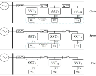
Figure 4.3 Controller implementation schemes ... 67

Figure 4.4 Block diagram of the decentralized controller implementation ... 69

Figure 4.5 Three SST test system ... 74

Figure 4.6 DAB output DC voltage of 𝑆𝑆𝑇1 ... 76

Figure 4.7 DAB output DC voltage of 𝑆𝑆𝑇₂ ... 77

Figure 4.8 DAB output DC voltage of 𝑆𝑆𝑇₃ ... 77

Figure 4.9 Input current of 𝑆𝑆𝑇₂ ... 78

Figure 4.10 Microgrid current of 𝑆𝑆𝑇₂ ... 78

Figure 4.11 Input current of 𝑆𝑆𝑇3 ... 79

Figure 4.12 Microgrid current of 𝑆𝑆𝑇₃ ... 79

Figure 4.13 Rectifier output DC voltage of 𝑆𝑆𝑇₁ ... 80

Figure 4.15 Rectifier output DC voltage of 𝑆𝑆𝑇3 ... 81

Figure 4.16 DAB output DC voltage of 𝑆𝑆𝑇2 in presence of saturation in microgrid current .... 82

Figure 4.17 Microgrid current of 𝑆𝑆𝑇₂ in presence of saturation in microgrid current ... 83

Figure 4.18 Input current of 𝑆𝑆𝑇₂ in presence of saturation in microgrid current ... 83

Figure 4.19 Duty cycle of the rectifier stage of 𝑆𝑆𝑇₂ with centralized/decentralized controller ... 84

Figure 4.20 Input current of 𝑆𝑆𝑇1 in black start mode ... 85

Figure 4.21 DAB output DC voltage of 𝑆𝑆𝑇1 in black start mode ... 85

Figure 5.1 FREEDM system in the islanded mode of operation ... 89

Figure 5.2 Feasibility circles of the master SST ... 92

Figure 5.3 Feasibility region expansion of the master SST ... 93

Figure 5.4 Low-voltage scaled SST testbed ... 95

Figure 5.5 Operation of 𝑆𝑆𝑇₂ in the islanded mode without help from master SST ... 95

Figure 5.6 Operation of 𝑆𝑆𝑇₃ in the islanded mode without help from master SST ... 96

Figure 5.7 Operation of 𝑆𝑆𝑇2 in the islanded mode with help from master SST ... 96

CHAPTER 1

INTRODUCTION

1.1. Research Background

The electrical energy consumption is rising globally. According to the United States Energy Information Administration, total US energy consumption in 2017 was over 97.4 quadrillion Btu (28.5 trillion kWh) [1]. Electric energy production heavily relies on coal, oil and natural gas; however, since these resources are finite and are destructing the earth, the need for new types of energy resources is increasing. Renewable energy resources are becoming more popular due to their reduced system costs and 𝐶𝑂₂ emission. Since 2009, system cost of onshore wind and solar photovoltaics (PV) have reduced by 14% and 61%, respectively [1]. Moreover, compared with natural gas, which emits between 0.6 and 2 and coal, which emits between 1.4 and 3.6 pounds of 𝐶𝑂2⁄_𝑘𝑊ℎ, wind emits only 0.02 to 0.04

pounds of 𝐶𝑂2⁄_𝑘𝑊ℎ and solar emits 0.07 to 0.2 𝐶𝑂2⁄_𝑘𝑊ℎ [3, 4].

variable and unmanaged power sources which impacts the stability, reliability and efficiency of the power grid [8]. Some of the technical challenges of high PV penetration into the traditional power grid are reverse power flow from the feeder to the substation which results in overvoltage and higher loss in the lines [9, 10, 11], voltage fluctuations due to the change in solar irradiance [12] and voltage/current unbalance in multi-phase systems. Among these problems, voltage rise is the major issue due to unstabilizing the distribution network [13]. A lot of research has been conducted to solve this issue and solutions such as using static synchronous compensator (STATCOM), static VAR compensator (SVC), Volt-Var control (VVC), DC transmission and distribution systems, Volt-Watt control (VW) and storage systems have been proposed [14, 15, 16, 17, 18, 19, 20, 21, 22, 23, 24, 25, 26]. VAR compensators mitigate the voltage rise by injecting reactive power through switching capacitors into the system [14, 15]. Volt-Var control (VVC) is another method that can be used to reduce the voltage rise along the feeder by injecting reactive power and minimize the losses in the system which would increase the system efficiency and lifetime of the equipment [16, 17]. In volt-Watt control (VW), a high level of power may be curtailed in order to keep the voltage within the required limits [18]. Storage systems have lately been a popular solution to mitigate the voltage rise in distribution feeders. They can help buffer renewable energy generation, capturing a portion of the energy produced during light load and exporting it back to the network when required and therefore, no power curtailment will be necessary [19].

Management (FREEDM) systems center [27]. The one node FREEDM system consists of a solid-state transformer (SST), a DC microgrid and an AC microgrid. Each microgrid can consist of solar or wind DRERs, a DESD system and local loads. SST serves as an energy router and its voltage transformation is achieved through using a high frequency transformer which results in a smaller and lighter transformer compared with traditional transformers. Moreover, the SST system provides some functionalities that cannot be obtained using traditional transformers such as decoupling the low voltage side from the grid side, voltage sag restoration, power factor correction, fault current monitoring, power flow control, etc. [27, 28, 29].

Several research has been done on the functionalities, performance and application of SSTs in power distribution systems [27, 28, 29, 32, 33, 34, 35, 36, 37]. In [27, 28, 29], the concept of FREEDM system is proposed and advantages of this new generation of transformers compared to traditional transformers are explained. In [32], an average model of a single-phase SST using state-space averaging is derived and a control strategy for the SST is proposed. In [33], a power management strategy for a single SST system in presence of renewable energy systems is proposed. In [34], black start performance of a lab scale single SST system is investigated. In [35], some failures in the operation of a SST-based power distribution network is observed; however, the reason behind the failure is unknown. Unlike the traditional transformers, the SST system is modelled with differential equations and, therefore, aside from the physical bounds of the system dictated by its component ratings, there are some mathematical bounds on the system that define the feasible operational range of it. No study has been done on the mathematical operational bounds of the SST system. Moreover, in [36], a detailed model of a SST is derived and a stabilizing controller for the system based on its linearized model is designed. This controller does not guarantee asymptotic stability of the system (modelled through nonlinear dynamic equations). Furthermore, the controller may not work in a multi-SST based power distribution system. Feasibility analysis and an asymptotically stabilizing controller design for a multi-SST based power distribution network have been studied in this dissertation.

1.2. Research Motivation

improvements in the design of wide-band gap semiconductor devices, replacing the traditional transformers with SSTs is a valid option. Moreover, due to reduced use of copper and laminated steel in SSTs compared to traditional transformers, these systems are more cost-effective [32]. SST is an energy router that consists of three stages:

1. The front-end rectifier stage which is used to convert the grid side AC voltage into a DC voltage.

2. The dual-active bridge (DAB) converter that converts the high DC voltage at the output of the rectifier into a low DC voltage through a high frequency transformer. This low DC voltage is used as the common feeder for the DC microgrid.

3. The voltage source inverter which inverts the DC voltage at the output of the DAB into an AC voltage which is used as the common feeder for the AC microgrid.

FREEDM system, power flow equations must be resolved to find the new operating point of the system and update its references accordingly to maintain the feasibility. Therefore, knowledge about the power flow equations of the system seems necessary. Also, when the system enters the islanded mode of operation, one SST acts as the master and is responsible to regulate the common feeder voltage of the system while the other SSTs act as slaves and are responsible to deliver the required power to their corresponding loads. In this case, system references must be selected such that feeder voltage and power flow requirements are met while system maintains its feasibility constraints. Therefore, feasibility analysis on the islanded mode of operation needs to be studied. It should be noted that feasibility is a necessary but not sufficient condition to guarantee that the system will maintain its operation. Aside from providing feasible references to the system, the operating point also needs to be stable. Therefore, a controller must be designed for the system that would stabilize its operating point. Moreover, a region of attraction of the controller needs to be derived so that the operating point of the system is always chosen in that range.

1.3. Contribution

Main contributions of the work presented in this dissertation are listed below:

1. Nonlinear dynamical models for three stages of an SST (front-end rectifier, dual-active bridge converter and voltage source inverter) are developed.

presence of a change in the system is conducted. This analysis is validated in a three SST power distribution network.

3. A centralized controller based on the Lyapunov stability theory is proposed that guarantees asymptotic stability of a multi-SST based power distribution network. The controller is then simplified to design a decentralized controller where each SST only takes feedback from its own system states to stabilize the global system. A comparison on the performance of the centralized vs decentralized controller is provided. Moreover, stability of the system in presence of incorrect references in the controller is studied. This controller is validated in a three SST power distribution network.

4. Feasibility analysis of the FREEDM system in the islanded mode of operation is studied to provide feasible references for the “master” and “slave” SSTs. Moreover, the performance of the designed controller on the system in islanded mode of operation is investigated.

1.4. Dissertation Outline

The outline of the dissertation is as follows:

Chapter 2

developed model is built and different case studies such as changes in input grid voltage, load and microgrid output current are studied.

This analysis was presented in the IEEE Energy Conversion Congress and Expo (ECCE)’2016 and is also accepted in the IEEE Transactions on Industrial Applications Society (IAS) [40, 41].

Chapter 3

Based on the developed dynamic model, the feasible operating bounds of each sub-stage of the SST model is derived. A method to increase the feasible operating range of the SST is proposed based on its dynamic model and system parameters. These results are then extended for a multi-SST based power distribution system. To maintain system feasibility in presence of a system parameter/load change, a power flow analysis is conducted which facilitates updating the references in the system. These results are verified in a three SST power distribution system.

Results presented in this chapter are accepted in the IEEE Transactions on Power Systems (TPWRS) [39].

Chapter 4

the system in presence of incorrect references in the controller is studied. This controller is validated in a three SST power distribution network.

The analysis in this chapter is drafted to submit to the IEEE Transactions on power systems (TPWRS).

Chapter 5

Feasibility of the FREEDM system in the islanded mode of operation is studied in this chapter. When the grid gets disconnected from the FREEDM system, one SST will operate as the master and it will be responsible to maintain the feeder voltage at a desired value while the other SSTs will operate as slaves and continue their operation as in the grid-tied case. Finding proper references for the system to maintain its feasibility when it gets disconnected from the grid is the main focus of this chapter. Moreover, the performance of the proposed controller in Chapter 4 on the FREEDM system in islanded mode of operation is studied.

The analysis in this chapter is drafted to submit to IEEE Energy Conversion Congress and Expo (ECCE).

Chapter 6

CHAPTER 2

DYNAMIC MODELING OF A SOLID-STATE

TRANSFORMER BASED POWER DISTRIBUTION SYSTEM

2.1. Introduction

In this chapter, a physics-based dynamic model for a solid-state transformer (SST) based power distribution system is presented. The future distribution-level power system is envisioned to have SST as its centerpiece, as described in the Future Renewable Electric Energy Delivery and Management (FREEDM) system architecture [27]. The FREEDM system design is based on an energy router, i.e., the SST which connects distributed renewable energy resources (DRER), distributed energy storage devices (DESD) and local loads on the low voltage AC and DC side with the distribution grid. SST is a power electronics-based transformer where several layers of control, communications and intelligence are integrated into it for demand-side management, control of voltage and power factor, elimination of customer-side harmonics, and for providing low-voltage ride-through and low-frequency ride-through functionalities [42]. A key feature that distinguishes the SST from a traditional transformer is its ability to decouple and buffer medium-voltage distribution grids from the low-voltage feeder sections which is possible through a high frequency transformer [43].

as the common feeder for DC microgrid applications. The inverter is used to inverter the low DC voltage into a low AC voltage which is used as the common feeder for AC microgrid applications [44].

In this chapter, dynamic model for each of these stages are derived using the state-space averaging technique. Averaging provides a simpler way to model systems [45, 46]. Especially in power electronic converters, it helps avoid the need to include the high frequency PWM switching harmonics for system dynamic analysis [47, 48]. The complete model of a SST can be found by relating these individual stage models together through algebraic equations. This accumulated final model is used in the later chapters for feasibility study and controller design.

2.2. Solid-State Transformer Dynamic Model

+ -+ -DC MG + -+ -DAB RECTIFIER INVERTER Vin

Rrec1 Lrec1 Rrec2 Lrec2

Cf _Crec

Rs1

CDABin

LDAB _N:1

CDABout Rs2 Linv AC MG Cinv

Figure 2.1 Solid-state transformer circuit model.

2.2.1. Front-end Rectifier

The first stage in the SST system is the front-end rectifier which is used to connect the SST to the grid. This stage converts the high AC grid voltage into a high DC voltage. The proposed rectifier model has a LCL filter in its AC side and its circuit model is shown in Fig. 2.2. As it can be seen in this figure, states of the system are the currents of the grid-side and inverter-side inductors, voltage across the LCL filter capacitor and the output voltage of the rectifier across the DC side capacitor. Using the state-space averaging technique, the differential equations below represent the system in the phase domain.

𝐿𝑟𝑒𝑐1

𝑑𝑖_{𝐿𝑟𝑒𝑐1}

𝑑𝑡 (𝑡) = −𝑅𝑟𝑒𝑐1𝑖𝐿𝑟𝑒𝑐1(𝑡) + 𝑣𝐶𝑓(𝑡) − 𝑣𝑖𝑛(𝑡) (2.1)

𝐶𝑓

𝑑𝑣_𝐶𝑓

𝑑𝑡 (𝑡) = 𝑖𝐿𝑟𝑒𝑐2(𝑡) − 𝑖𝐿𝑟𝑒𝑐1(𝑡) (2.2)

𝐿𝑟𝑒𝑐2

𝑑𝑖_{𝐿𝑟𝑒𝑐2}

𝑑𝑡 (𝑡) = −𝑅𝑟𝑒𝑐2𝑖𝐿𝑟𝑒𝑐2(𝑡) − 𝑣𝐶𝑓(𝑡) + 𝑑𝑟𝑒𝑐(𝑡)𝑣𝐶𝑟𝑒𝑐(𝑡) (2.3)

𝐶𝑟𝑒𝑐

𝑑𝑣_{𝐶𝑟𝑒𝑐}

𝑑𝑡 (𝑡) = − 1 𝑅𝐿,𝑟𝑒𝑐(𝑡)

+

-Vin

Rrec1 Lrec1 Rrec2 Lrec2

C

+

-Figure 2.2 Front-end rectifier circuit.

In order to make the analysis simpler, d-q transformation can be used to represent the AC states by two DC components. For single phase d-q transformation, first, an imaginary phase which is lagging the original phase by 90 degrees is defined (denoted by m) and then, d-q transformation given in equation (2.5) is used to find the transformed dynamic model [50]. The final rectifier model in the new coordinates is presented in equations (2.7)-(2.13). In these equations, the time argument components have been eliminated for simplicity.

[𝑥_𝑥𝑑

𝑞] = [

sin(𝜃) −cos(𝜃) cos (𝜃) sin(𝜃) ] [

𝑥_𝑎

𝑥_𝑚] (2.5)

𝜃̇ = 𝜔 (2.6)

𝐿𝑟𝑒𝑐1

𝑑𝑖_{𝐿𝑟𝑒𝑐1,𝑑}

𝑑𝑡 = −𝑅𝑟𝑒𝑐1𝑖𝐿𝑟𝑒𝑐1,𝑑+ 𝜔𝐿𝑟𝑒𝑐1𝑖𝐿𝑟𝑒𝑐1,𝑞+ 𝑣𝐶𝑓,𝑑− 𝑣𝑖𝑛,𝑑 (2.7)

𝐿_{𝑟𝑒𝑐1}𝑑𝑖𝐿𝑟𝑒𝑐1,𝑞

𝑑𝑡 = −𝜔𝐿𝑟𝑒𝑐1𝑖𝐿𝑟𝑒𝑐1,𝑑− 𝑅𝑟𝑒𝑐1𝑖𝐿𝑟𝑒𝑐1,𝑞 + 𝑣𝐶𝑓,𝑞− 𝑣𝑖𝑛,𝑞 (2.8)

𝐶𝑓

𝑑𝑣𝐶𝑓,𝑑

𝑑𝑡 = 𝑖𝐿𝑟𝑒𝑐2,𝑑− 𝑖𝐿𝑟𝑒𝑐1,𝑑+ 𝜔𝐶𝑓𝑣𝐶𝑓,𝑞 (2.9)

𝐶𝑓

𝑑𝑣_{𝐶𝑓,𝑞}

𝑑𝑡 = 𝑖𝐿𝑟𝑒𝑐2,𝑞− 𝑖𝐿𝑟𝑒𝑐1,𝑞− 𝜔𝐶𝑓𝑣𝐶𝑓,𝑑 (2.10)

𝐿𝑟𝑒𝑐2

𝑑𝑖_{𝐿𝑟𝑒𝑐2,𝑑}

𝐿𝑟𝑒𝑐2

𝑑𝑖_{𝐿𝑟𝑒𝑐2,𝑞}

𝑑𝑡 = −𝜔𝐿𝑟𝑒𝑐2𝑖𝐿𝑟𝑒𝑐2,𝑑− 𝑅𝑟𝑒𝑐2𝑖𝐿𝑟𝑒𝑐2,𝑞 − 𝑣𝐶𝑓,𝑞+ 𝑑𝑟𝑒𝑐,𝑞𝑣𝐶𝑟𝑒𝑐 (2.12)

𝐶𝑟𝑒𝑐

𝑑𝑣_{𝐶𝑟𝑒𝑐} 𝑑𝑡 = −

1

2𝑑𝑟𝑒𝑐,𝑑𝑖𝐿𝑟𝑒𝑐2,𝑑−

1

2𝑑𝑟𝑒𝑐,𝑞𝑖𝐿𝑟𝑒𝑐2,𝑞 −

1 𝑅𝐿,𝑟𝑒𝑐

𝑣𝐶𝑟𝑒𝑐

+1

2(𝑑𝑟𝑒𝑐,𝑞𝑖𝐿𝑟𝑒𝑐2,𝑞− 𝑑𝑟𝑒𝑐,𝑑𝑖𝐿𝑟𝑒𝑐2,𝑑) cos(2𝜃)

−1

2(𝑑𝑟𝑒𝑐,𝑑𝑖𝐿𝑟𝑒𝑐2,𝑞+ 𝑑𝑟𝑒𝑐,𝑞𝑖𝐿𝑟𝑒𝑐2,𝑑) sin(2𝜃) (2.13)

Conventionally, the output DC voltage of the rectifier is controlled using the duty cycle of the H-bridge in the rectifier circuit using an outer-loop voltage controller and an inner-loop d-axis current controller. Moreover, reactive power flow through the rectifier can be controlled by controlling the q-axis input current [51, 52]. A unity power factor can be achieved by setting the reference for the q-axis input current equal to zero [53]. The dynamic model of the aforementioned controller using PI controllers is presented below:

ξ̇₁ = 𝑣_{𝐶𝑟𝑒𝑐,𝑟𝑒𝑓}− 𝑣_{𝐶𝑟𝑒𝑐} (2.14)

ξ̇2 = 𝐾𝑃1(𝑣𝐶𝑟𝑒𝑐,𝑟𝑒𝑓− 𝑣𝐶𝑟𝑒𝑐) + 𝐾𝐼1ξ1− 𝑖𝐿𝑟𝑒𝑐2,𝑑 (2.15)

ξ̇₃ = 𝑖_{𝐿𝑟𝑒𝑐2,𝑞,𝑟𝑒𝑓}− 𝑖_{𝐿𝑟𝑒𝑐2,𝑞} (2.16)

The output signals of this control system are the d-axis and q-axis duty cycle of the rectifier and their equations are given below.

𝑑_{𝑟𝑒𝑐,𝑑} = 𝐾_𝑃2(𝐾_𝑃1(𝑣_{𝐶𝑟𝑒𝑐,𝑟𝑒𝑓}− 𝑣_{𝐶𝑟𝑒𝑐}) + 𝐾_𝐼1ξ₁− 𝑖_{𝐿𝑟𝑒𝑐2,𝑑}) + 𝐾_𝐼2ξ₂ (2.17)

𝑑_{𝑟𝑒𝑐,𝑞} = 𝐾_𝑃3(𝑖_{𝐿𝑟𝑒𝑐2,𝑞,𝑟𝑒𝑓}− 𝑖_{𝐿𝑟𝑒𝑐2,𝑞}) + 𝐾_𝐼3ξ₃ (2.18)

The control system gains must be designed such that ∀𝑡 ≥ 0, the following condition is satisfied.

𝑑_{𝑟𝑒𝑐,𝑑}2 + 𝑑𝑟𝑒𝑐,𝑞2 ≤ 1 (2.19)

PI

-+

+

_-

PI

v

v

i

d

PI

-+

i

i

d

Figure 2.3 Rectifier nested PI controller scheme.

An approximate model for the rectifier model can be achieved by eliminating the dynamics of the LCL filter capacitor. Since 𝐶𝑓 is very small, singular perturbation can be

used to simplify the model and represent the filter as an inductor in series with a resistor. Therefore, by defining 𝐿_𝑟𝑒𝑐 = 𝐿_{𝑟𝑒𝑐1}+ 𝐿_{𝑟𝑒𝑐2} and 𝑅_𝑟𝑒𝑐 = 𝑅_{𝑟𝑒𝑐1}+ 𝑅_{𝑟𝑒𝑐2}, the model can be simplified as:

𝐿𝑟𝑒𝑐

𝑑𝑖_{𝐿𝑟𝑒𝑐,𝑑}

𝑑𝑡 = −𝑅𝑟𝑒𝑐𝑖𝐿𝑟𝑒𝑐,𝑑+ 𝜔𝐿𝑟𝑒𝑐𝑖𝐿𝑟𝑒𝑐,𝑞 + 𝑑𝑟𝑒𝑐,𝑑𝑣𝐶𝑟𝑒𝑐 − 𝑣𝑖𝑛,𝑑 (2.20)

𝐿_𝑟𝑒𝑐𝑑𝑖𝐿𝑟𝑒𝑐,𝑞

𝑑𝑡 = −𝜔𝐿𝑟𝑒𝑐𝑖𝐿𝑟𝑒𝑐,𝑑− 𝑅𝑟𝑒𝑐𝑖𝐿𝑟𝑒𝑐,𝑞+ 𝑑𝑟𝑒𝑐,𝑞𝑣𝐶𝑟𝑒𝑐 − 𝑣𝑖𝑛,𝑞 (2.21)

𝐶𝑟𝑒𝑐

𝑑𝑣_{𝐶𝑟𝑒𝑐} 𝑑𝑡 = −

1

2𝑑𝑟𝑒𝑐,𝑑𝑖𝐿𝑟𝑒𝑐,𝑑−

1

2𝑑𝑟𝑒𝑐,𝑞𝑖𝐿𝑟𝑒𝑐,𝑞−

1 𝑅𝐿,𝑟𝑒𝑐

𝑣𝐶𝑟𝑒𝑐

+1

2(𝑑𝑟𝑒𝑐,𝑞𝑖𝐿𝑟𝑒𝑐,𝑞− 𝑑𝑟𝑒𝑐,𝑑𝑖𝐿𝑟𝑒𝑐,𝑑) cos(2𝜃)

−1

2.2.2. Dual-Active Bridge Converter

Dual-active bridge (DAB) converter is the second stage of a SST system. In this stage, the high DC voltage at the output of the rectifier is converted to a low DC voltage which can be used for DC microgrid applications. The circuit diagram of a DAB is shown in Fig. 2.4. As it can be seen in this figure, DAB consists of two H-bridges with a high frequency transformer in between these two bridges. In order to transfer the power from one side to the other, phase difference must exist between the switching of these bridges. The states of the DAB system are input capacitor voltage, output capacitor voltage and current of the transformer inductor. However, since the inductor current state is much faster than the two capacitor voltage states, singular perturbation can be used to present the system using only two states. The inductor current of DAB is approximated linearly as a function of two capacitor voltage states and DAB parameters [54, 55]. This would result in the following dynamic model for DAB:

𝐶_{𝐷𝐴𝐵,𝑖𝑛}𝑑𝑣𝐶𝐷𝐴𝐵,𝑖𝑛

𝑑𝑡 =

1

𝑅_𝑠1𝑣𝐶𝑟𝑒𝑐−

1

𝑅_𝑠1𝑣𝐶𝐷𝐴𝐵,𝑖𝑛−

𝑑_𝐷𝐴𝐵(1 − 𝑑𝐷𝐴𝐵)𝑁

2𝑓_𝑠𝐿_𝐷𝐴𝐵 𝑣𝐶𝐷𝐴𝐵,𝑜𝑢𝑡 (2.23)

𝐶_{𝐷𝐴𝐵,𝑜𝑢𝑡}𝑑𝑣𝐶𝐷𝐴𝐵,𝑜𝑢𝑡

𝑑𝑡 =

𝑑𝐷𝐴𝐵(1 − 𝑑𝐷𝐴𝐵)𝑁

2𝑓𝑠𝐿𝐷𝐴𝐵

𝑣_{𝐶𝐷𝐴𝐵,𝑖𝑛}− 1 𝐿𝐷𝐶

𝑣_{𝐶𝐷𝐴𝐵,𝑜𝑢𝑡} (2.24)

In the equations above, 𝐶_{𝐷𝐴𝐵,𝑖𝑛}, 𝐶_{𝐷𝐴𝐵,𝑜𝑢𝑡}, 𝑅_𝑠1, 𝑁, 𝑓_𝑠 and 𝐿_𝐷𝐴𝐵 represent the DAB input

+

-DC

MG

+

-VCrec

Rs1

CDABin

LDAB _N:1

CDABout

Figure 2.4 Dual-active bridge circuit.

The output DC voltage of DAB is controlled using the phase shift between the H-bridges in the system [56]. The control system equations for this purpose using a PI controller are given below.

ξ̇₄ = 𝑣_{𝐶𝐷𝐴𝐵,𝑜𝑢𝑡,𝑟𝑒𝑓}− 𝑣_{𝐶𝐷𝐴𝐵,𝑜𝑢𝑡} (2.25)

𝑑𝐷𝐴𝐵 = 𝐾𝑃4(𝑣𝐶𝐷𝐴𝐵,𝑜𝑢𝑡,𝑟𝑒𝑓− 𝑣𝐶𝐷𝐴𝐵,𝑜𝑢𝑡) + 𝐾𝐼4ξ4 (2.26)

The control system gains must be designed such that ∀𝑡 ≥ 0, the following inequality

is satisfied.

−1 ≤ 𝑑𝐷𝐴𝐵 ≤ 1 (2.27)

The control system for DAB system is presented in Fig. 2.5.

PI

-+

v

d

v

2.2.3. Voltage Source Inverter

Inverter is the last stage of the SST system which is used to invert the output DC voltage of the DAB into an AC voltage which can be used for AC microgrid applications. The circuit diagram of the inverter stage is shown in Fig. 2.6. Inductor current and capacitor voltage of the output filter are the states of this subsystem. Similar to the front-end rectifier stage, d-q transformation can be used to derive the dynamic model of the inverter.

+

-Vin,inv

Rs2

Linv

AC

MG Cinv

Figure 2.6 Voltage source inverter circuit.

𝐿𝑖𝑛𝑣

𝑑𝑖_{𝐿𝑖𝑛𝑣,𝑑}

𝑑𝑡 = 𝑑𝑖𝑛𝑣,𝑑𝑣𝑖𝑛,𝑖𝑛𝑣− 𝑅𝑠2𝑖𝐿𝑖𝑛𝑣,𝑑+ Ω𝐿𝑖𝑛𝑣𝑖𝐿𝑖𝑛𝑣,𝑞− 𝑣𝐶𝑖𝑛𝑣,𝑑 (2.28)

𝐿_𝑖𝑛𝑣𝑑𝑖𝐿𝑖𝑛𝑣,𝑞

𝑑𝑡 = 𝑑𝑖𝑛𝑣,𝑞𝑣𝑖𝑛,𝑖𝑛𝑣− Ω𝐿𝑖𝑛𝑣𝑖𝐿𝑖𝑛𝑣,𝑑− 𝑅𝑠2𝑖𝐿𝑖𝑛𝑣,𝑞− 𝑣𝐶𝑖𝑛𝑣,𝑞 (2.29)

𝐶_𝑖𝑛𝑣𝑑𝑣𝐶𝑖𝑛𝑣,𝑑

𝑑𝑡 = 𝑖𝐿𝑖𝑛𝑣,𝑑−

1

𝐿_𝑎𝑐𝑣𝐶𝑖𝑛𝑣,𝑑+ Ω𝐶𝑖𝑛𝑣𝑣𝐶𝑖𝑛𝑣,𝑞 (2.30)

𝐶𝑖𝑛𝑣

𝑑𝑣_{𝐶𝑖𝑛𝑣,𝑞}

𝑑𝑡 = 𝑖𝐿𝑖𝑛𝑣,𝑞− Ω𝐶𝑖𝑛𝑣𝑣𝐶𝑖𝑛𝑣,𝑑−

1 𝐿𝑎𝑐

In the equations above, 𝐿𝑖𝑛𝑣, 𝐶𝑖𝑛𝑣, Ω and 𝑅𝑠2 represent the inverter output filter

inductor, output filter capacitor, output signal frequency and the resistor connecting DAB and inverter, respectively.

The inverter controller regulates its output voltage at a desired level by controlling the d-axis and q-axis output voltage [57]. Dynamic equations representing the PI based controller for the inverter are shown below.

ξ̇₅ = 𝑣_{𝐶𝑖𝑛𝑣,𝑑,𝑟𝑒𝑓}− 𝑣_{𝐶𝑖𝑛𝑣,𝑑} (2.32)

ξ̇6 = 𝑣𝐶𝑖𝑛𝑣,𝑞,𝑟𝑒𝑓− 𝑣𝐶𝑖𝑛𝑣,𝑞 (2.33)

𝑑𝑖𝑛𝑣,𝑑 = 𝐾𝑃5(𝑣𝐶𝑖𝑛𝑣,𝑑,𝑟𝑒𝑓− 𝑣𝐶𝑖𝑛𝑣,𝑑) + 𝐾𝐼5ξ5 (2.34)

𝑑_{𝑖𝑛𝑣,𝑞} = 𝐾_𝑃6(𝑣_{𝐶𝑖𝑛𝑣,𝑞,𝑟𝑒𝑓}− 𝑣_{𝐶𝑖𝑛𝑣,𝑞}) + 𝐾_𝐼6ξ₆ (2.35)

The control system gains must be designed such that ∀𝑡 ≥ 0, the following condition is satisfied.

𝑑_{𝑖𝑛𝑣,𝑑}2 + 𝑑_{𝑖𝑛𝑣,𝑞}2 ≤ 1 (2.36)

The PI based controller for the inverter system is presented in Fig. 2.7.

PI

-+

v

d

v

PI

-+

v

d

v

2.2.4. Overall SST Model

Let 𝑥𝑝 ∈ 𝑅19 denote the vector of state variables for all three stages of an SST. From

circuit calculations, 𝑅𝐿,𝑟𝑒𝑐 can be expressed as:

𝑅𝐿,𝑟𝑒𝑐 =

𝑣_{𝐶,𝑟𝑒𝑐}2 𝑣_𝐶2_{𝐷𝐴𝐵,𝑜𝑢𝑡}

𝐿𝐷𝐶 +

(𝑣_{𝐶,𝑟𝑒𝑐}− 𝑣_{𝐶𝐷𝐴𝐵,𝑖𝑛})2

𝑅𝑠1

(2.37)

The expression above accumulates for the losses and net loads seen by the SST system. Based on equations (2.1)-(2.36), the overall SST model can be written in a compact form as:

𝑥̇_𝑝(𝑡) = 𝑓1(𝑥𝑝(𝑡), 𝛼1, 𝛼2, 𝐿𝑑𝑐, 𝐿𝑎𝑐) + 𝑓2(𝑥𝑝(𝑡), cos(𝜃(𝑡)) , sin(𝜃(𝑡))) (2.38)

𝑔(𝑥_𝑝(𝑡), 𝛼1, 𝛼2, 𝐿𝑑𝑐, 𝐿𝑎𝑐) ≤ 0 (2.39)

Where 𝛼₁ and 𝛼₂ represent the set of system parameters and references, respectively. The function 𝑓2(. ) models the second harmonic effect of 𝑥𝑝(𝑡) following from the last two

terms in equation (2.13). Moreover, function 𝑔(. ) models the three duty cycle equations given for each subsystem.

2.2.5. DC and AC Microgrids

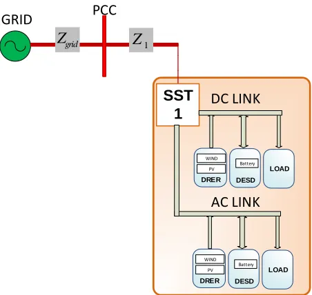
Each of these interface circuits are responsible for voltage rectifying, inverting or boosting [59, 60]. For example, the interface circuit that connects solar DRER to the DC feeder is a boost converter that guarantees DRER operation at its maximum power point [61]. The SST system should operate in a plug-and play manner meaning that connecting/disconnecting any of these microgrid subsystems should not have any effect on the operation of the system and the system must keep running. In Fig. 2.8, a single SST system with its DC and AC microgrids are shown.

GRID

DESD

Battery

SST 1

DRER

WIND

PV LOAD

DESD

Battery

DRER

WIND

PV LOAD

DC LINK

AC LINK grid

Z Z₁

PCC

Figure 2.8 Single SST FREEDM system.

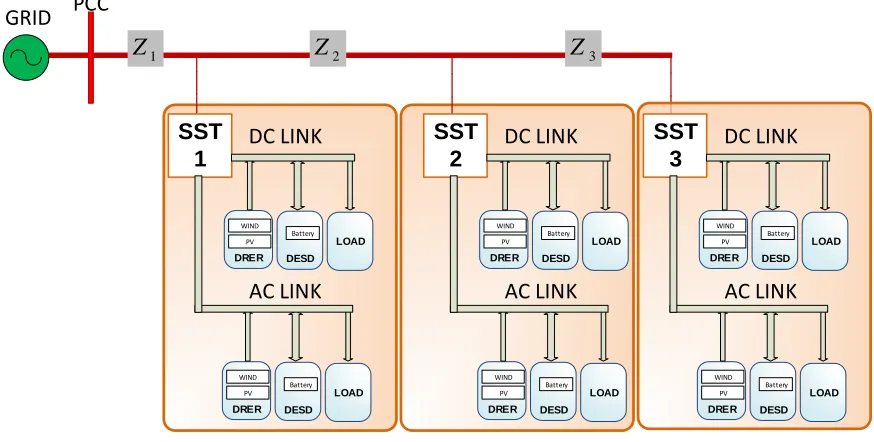
2.3. Multi-SST FREEDM Dynamic Model

be used to relate each SST’s model to the other ones. Equations for d-axis and q-axis input voltage of the 𝑖𝑡ℎ SST is shown in equations (2.40) and (2.41), respectively. In these equations, 𝑍_𝑘= 𝑅_𝑘+ 𝑗𝑋_𝑘 represents the impedance of the distribution line between the (𝑘 − 1)𝑡ℎ and 𝑘𝑡ℎ SST, respectively (𝑍1 represents the impedance of the distribution line

between the grid and first SST in the network).

DESD Battery SST 3 DRER WIND PV GRID LOAD DESD Battery DRER WIND PV LOAD DC LINK AC LINK DESD Battery SST 2 DRER WIND PV LOAD DESD Battery DRER WIND PV LOAD DC LINK AC LINK DESD Battery SST 1 DRER WIND PV LOAD DESD Battery DRER WIND PV LOAD DC LINK AC LINK 1

Z Z₂ Z₃

PCC

Figure 2.9 Multi-SST FREEDM system.

𝑣_{𝑖𝑛,𝑑𝑖} = ∑ 𝑅_𝑘

𝑖

𝑘=1

∑ 𝑖_{𝐿𝑟𝑒𝑐1,𝑑𝑗}

𝑛

𝑗≥𝑘

− ∑ 𝑋_𝑘

𝑖

𝑘=1

∑ 𝑖_{𝐿𝑟𝑒𝑐1,𝑞𝑗}

𝑛 𝑗≥𝑘 (2.40) 𝑣_{𝑖𝑛,𝑞𝑖} = ∑ 𝑋_𝑘 𝑖 𝑘=1

∑ 𝑖_{𝐿𝑟𝑒𝑐1,𝑑𝑗}

𝑛

𝑗≥𝑘

+ ∑ 𝑅_𝑘

𝑖

𝑘=1

∑ 𝑖_{𝐿𝑟𝑒𝑐1,𝑞𝑗}

𝑛

𝑗≥𝑘

(2.41)

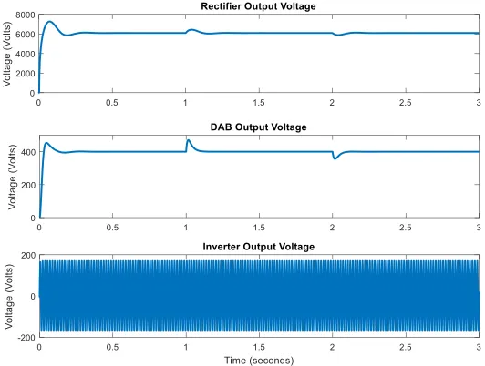
2.4. Case Studies and Simulation Results

goal of the local controller is to regulate the output voltage of rectifier, DAB and inverter along with the input current of SST. Fig. 2.10 shows the rectifier, DAB and inverter output voltages when the DC link load is 80 𝛺 and the AC link is 50 < 53𝑜 𝛺. Moreover, Fig. 2.11 shows the SST input current. At first, there is no current from the microgrids. As it can be seen in the figure, local controllers are able to regulate the voltages and input current to their steady state value. At 𝑡 = 1 𝑠𝑒𝑐, DC microgrid current changes from 0 𝐴 to 5 𝐴 (can be regarded as discharging of the battery or increase in renewable energy power). The extra current from the DC microgrid results in a reduction in the input current from the grid. Moreover, there is an increase in the rectifier and DAB output voltage. However, the local controllers are able to regulate the voltages back to their steady-state. At 𝑡 = 2 𝑠𝑒𝑐, the AC link microgrid current changes from 0 𝐴 to −15 𝐴 (can be regarded as charging of the battery or decrease in renewable energy power). After a sag in the voltages, the controllers regulate the voltage and current values back to their references. As it can be seen in the figures, the effect of these changes on inverter voltage is very small. Fig. 2.12 shows the resulting dynamics in the input current at 𝑡 = 1 𝑠𝑒𝑐 (left) and 𝑡 = 2 𝑠𝑒𝑐 (right) more precisely.

Figure 2.11 SST input current under microgrid current variation.

Figure 2.12 SST input current dynamics under microgrid current variation.

Figure 2.13 SST dynamic performance under load variation.

The performance of the model is also observed for a change in grid impedance. Fig. 2.14 and Fig. 2.15 show the response of the system after a 50% increase in grid impedance at 𝑡 = 1 𝑠𝑒𝑐 and a 10% increase in grid voltage at 𝑡 = 2 𝑠𝑒𝑐. Moreover, in order to see the

Figure 2.14 SST dynamic performance under grid variation.

Figure 2.16 SST dynamic performance under changes in other SSTs.

2.5. Conclusion

CHAPTER 3

Feasibility Analysis of the FREEDM System

3.1. Introduction

As it was shown in the previous chapter, the average dynamic model of a SST is described by significantly nonlinear dynamics. Because of these nonlinearities, determining the “safe zones of operation” of distribution system models integrated with SSTs is an important problem. Unlike the traditional electric power system where automatic generation control (AGC) is used to adjust the power output of multiple generators at different power plants to match the changes in the load, in the concept of FREEDM system, the active and reactive power balances are realized through control of converters with appropriate choices for voltage and current references [62]. These references parametrize the nonlinear model of the SST, and therefore, it is critically important for grid operators to know the suitable combinations of voltage and current references that result in a feasible equilibria. Motivated by this interest, in this chapter, a set of analytical conditions that determine the feasibility conditions for the equilibria of SST models when they are connected to the distribution grid is derived. The analysis is first presented for a single SST system, and then, extended to systems with multiple SSTs connected in a tree topology. In some extreme cases, where the load of an SST goes beyond the allowable feasible range, tuning the system references will expand the feasibility range of the SST and therefore, make this new operating point, a feasible one. In this chapter, a method to expand the feasible operating range of the SST is proposed.

flow must be solved to find the new operating point of the system and provide appropriate references, accordingly. An analysis on the power flow solution of the FREEDM system is provided in this chapter. Based on this analysis, several methods can be proposed by which multiple SSTs can share a given change in load by generating an appropriate set of feasible references. Two of these methods which are proposed in [39] are discussed in this chapter. The approach is comparable to maintaining transient stability in transmission-level power systems. Transient stability analysis of a single machine infinite-bus power system, for example, shows that a synchronous generator has two feasible equilibria for a given load where one of these equilibria is stable and the other one is unstable. The system is always ensured to operate at the stable equilibrium by maintaining the system frequency at the synchronous value using Automatic Generation Control (AGC). The equilibrium conditions for distribution system models driven by SSTs, however, are far more complicated than in AGC; this is because the turbine references in synchronous generator models enter only as exogenous inputs whereas the references in SST models enter the dynamics directly through the states. This analysis is validated in a 3 SST power distribution system.

3.2. Single SST Feasibility Analysis

As it was discussed in chapter 2, the overall SST dynamic model can be written in a compact form as:

𝑥̇𝑝(𝑡) = 𝑓1(𝑥𝑝(𝑡), 𝛼1, 𝛼2, 𝐿𝑑𝑐, 𝐿𝑎𝑐) + 𝑓2(𝑥𝑝(𝑡), cos(𝜃(𝑡)) , sin(𝜃(𝑡))) (3.1)

𝑔(𝑥𝑝(𝑡), 𝛼1, 𝛼2, 𝐿𝑑𝑐, 𝐿𝑎𝑐) ≤ 0 (3.2)

Where 𝛼1 and 𝛼2 represent the set of system parameters and references, respectively.

of a time-varying sinusoidal function superimposed on top of a DC value. These DC values, in order, are given by the equilibrium of the vector 𝑥𝑓 ∈ 𝑅19 that satisfies:

𝑥̇_𝑓(𝑡) = 𝑓1(𝑥𝑓(𝑡), 𝛼1, 𝛼2, 𝐿𝑑𝑐, 𝐿𝑎𝑐) (3.3)

𝑔(𝑥_𝑓(𝑡), 𝛼1, 𝛼2, 𝐿𝑑𝑐, 𝐿𝑎𝑐) ≤ 0 (3.4)

The subscript f in the equation above stands for “fundamental” frequency component of the signals. For equilibrium analysis, only this fundamental component is of interest. Our discussion, therefore, is based on the model given in equations (3.3) and (3.4).

Let 𝑥∗ ∈ 𝑅19 be an equilibrium of the nonlinear differential-algebraic model given in equations (3.3) and (3.4), which implies that:

𝑓1(𝑥∗, 𝛼1, 𝛼2, 𝛼3) = 0 (3.5)

𝑔(𝑥∗, 𝛼₁, 𝛼₂, 𝛼₃) ≤ 0 (3.6)

Where 𝛼₃ represents the net constant DC and AC loads, namely 𝐿_𝑑𝑐 and 𝐿_𝑎𝑐, respectively. For a given set of model parameters and loads, one would wish to determine the voltage and current references in 𝛼2 so that equations (3.5) and (3.6) admit a real solution for

𝑥∗. Note that this solution may be non-unique, as discussed later. One would also wish to determine how the references in 𝛼₂ should be tuned to maintain the feasibility of the equilibrium 𝑥∗ _{when the loads are changed. Accordingly, the two problems of interest are}

defined as follows: Problem 1:

Problem 2:

Considering 𝛼₁ to be fixed, derive an algorithm on how the reference references in 𝛼₂ must be tuned in response to both predicted and unpredicted changes in the loads in 𝛼₃ for guaranteeing a real solution 𝑥∗ for equations (3.5) and (3.6).

In order to answer these questions, the expressions for the equilibria for each stage of the SST are derived next. For simplicity, the symbol 𝑥_𝑖 is used instead of 𝑥_𝑖∗ to denote the equilibrium value of the 𝑖𝑡ℎ state of the system. Note that this 𝑥𝑖 contains the equilibrium

information of only the fundamental component of the phasor, and should not be confused with the 𝑖𝑡ℎ state of the model given in equations (3.1) and (3.2), which contains both fundamental and second harmonics. Also, 𝑥_𝑖 can be non-unique, as will be seen in the following sections.

3.2.1. Feasibility Analysis of Rectifier

The dynamic model of the front-end rectifier stage was derived in chapter 2. By eliminating the second harmonic terms from the equations, the simplified dynamic model is as follows:

𝐿𝑟𝑒𝑐1

𝑑𝑖_{𝐿𝑟𝑒𝑐1,𝑑}

𝑑𝑡 = −𝑅𝑟𝑒𝑐1𝑖𝐿𝑟𝑒𝑐1,𝑑+ 𝜔𝐿𝑟𝑒𝑐1𝑖𝐿𝑟𝑒𝑐1,𝑞+ 𝑣𝐶𝑓,𝑑− 𝑣𝑖𝑛,𝑑 (3.7)

𝐿𝑟𝑒𝑐1

𝑑𝑖_{𝐿𝑟𝑒𝑐1,𝑞}

𝑑𝑡 = −𝜔𝐿𝑟𝑒𝑐1𝑖𝐿𝑟𝑒𝑐1,𝑑− 𝑅𝑟𝑒𝑐1𝑖𝐿𝑟𝑒𝑐1,𝑞 + 𝑣𝐶𝑓,𝑞− 𝑣𝑖𝑛,𝑞 (3.8)

𝐶_𝑓𝑑𝑣𝐶𝑓,𝑑

𝑑𝑡 = 𝑖𝐿𝑟𝑒𝑐2,𝑑− 𝑖𝐿𝑟𝑒𝑐1,𝑑+ 𝜔𝐶𝑓𝑣𝐶𝑓,𝑞 (3.9)

𝐶_𝑓𝑑𝑣𝐶𝑓,𝑞

𝑑𝑡 = 𝑖𝐿𝑟𝑒𝑐2,𝑞− 𝑖𝐿𝑟𝑒𝑐1,𝑞− 𝜔𝐶𝑓𝑣𝐶𝑓,𝑑 (3.10)

𝐿𝑟𝑒𝑐2

𝑑𝑖_{𝐿𝑟𝑒𝑐2,𝑑}

𝐿𝑟𝑒𝑐2

𝑑𝑖_{𝐿𝑟𝑒𝑐2,𝑞}

𝑑𝑡 = −𝜔𝐿𝑟𝑒𝑐2𝑖𝐿𝑟𝑒𝑐2,𝑑− 𝑅𝑟𝑒𝑐2𝑖𝐿𝑟𝑒𝑐2,𝑞 − 𝑣𝐶𝑓,𝑞+ 𝑑𝑟𝑒𝑐,𝑞𝑣𝐶𝑟𝑒𝑐 (3.12)

𝐶𝑟𝑒𝑐

𝑑𝑣_{𝐶𝑟𝑒𝑐} 𝑑𝑡 = −

1

2𝑑𝑟𝑒𝑐,𝑑𝑖𝐿𝑟𝑒𝑐2,𝑑−

1

2𝑑𝑟𝑒𝑐,𝑞𝑖𝐿𝑟𝑒𝑐2,𝑞 −

1 𝑅𝐿,𝑟𝑒𝑐

𝑣𝐶𝑟𝑒𝑐 (3.13)

ξ̇₁ = 𝑣_{𝐶𝑟𝑒𝑐,𝑟𝑒𝑓}− 𝑣_{𝐶𝑟𝑒𝑐} (3.14)

ξ̇₂ = 𝐾_𝑃1(𝑣_{𝐶𝑟𝑒𝑐,𝑟𝑒𝑓}− 𝑣_{𝐶𝑟𝑒𝑐}) + 𝐾_𝐼1ξ₁− 𝑖_{𝐿𝑟𝑒𝑐1,𝑑} (3.15)

ξ̇3 = 𝑖𝐿𝑟𝑒𝑐1,𝑞,𝑟𝑒𝑓− 𝑖𝐿𝑟𝑒𝑐1,𝑞 (3.16)

The equilibrium point of the rectifier system can be found by setting the right hand side of the equations above equal to zero. From dynamics of the controller equations in the steady state, 𝑣_{𝐶𝑟𝑒𝑐} = 𝑣_{𝐶𝑟𝑒𝑐,𝑟𝑒𝑓} and 𝑖_{𝐿𝑟𝑒𝑐1,𝑞} = 𝑖_{𝐿𝑟𝑒𝑐1,𝑞,𝑟𝑒𝑓}. Moreover, from equations (3.11) and (3.12):

𝑑_{𝑟𝑒𝑐,𝑑}𝑣_{𝐶𝑟𝑒𝑐} = 𝑅_{𝑟𝑒𝑐2}𝑖_{𝐿𝑟𝑒𝑐2,𝑑}− 𝜔𝐿_{𝑟𝑒𝑐2}𝑖_{𝐿𝑟𝑒𝑐2,𝑞} + 𝑣_{𝐶𝑓,𝑑} (3.17)

𝑑_{𝑟𝑒𝑐,𝑞}𝑣_{𝐶𝑟𝑒𝑐} = 𝜔𝐿_{𝑟𝑒𝑐2}𝑖_{𝐿𝑟𝑒𝑐2,𝑑}+ 𝑅_{𝑟𝑒𝑐2}𝑖_{𝐿𝑟𝑒𝑐2,𝑞}+ 𝑣_{𝐶𝑓,𝑞} (3.18)

Using these results in equation (3.13) −1

2𝑑𝑟𝑒𝑐,𝑑𝑖𝐿𝑟𝑒𝑐2,𝑑−

1

2𝑑𝑟𝑒𝑐,𝑞𝑖𝐿𝑟𝑒𝑐2,𝑞−

1 𝑅𝐿,𝑟𝑒𝑐

𝑣𝐶𝑟𝑒𝑐 = 0

→ 𝑑𝑟𝑒𝑐,𝑑𝑣𝐶𝑟𝑒𝑐𝑖𝐿𝑟𝑒𝑐2,𝑑+ 𝑑𝑟𝑒𝑐,𝑞𝑣𝐶𝑟𝑒𝑐𝑖𝐿𝑟𝑒𝑐2,𝑞 +

2 𝑅𝐿,𝑟𝑒𝑐

𝑣_𝐶2_𝑟𝑒𝑐 = 0

→ (𝑅_{𝑟𝑒𝑐2}𝑖_{𝐿𝑟𝑒𝑐2,𝑑}− 𝜔𝐿_{𝑟𝑒𝑐2}𝑖_{𝐿𝑟𝑒𝑐2,𝑞} + 𝑣_{𝐶𝑓,𝑑}) 𝑖_{𝐿𝑟𝑒𝑐2,𝑑}

+ (𝜔𝐿_{𝑟𝑒𝑐2}𝑖_{𝐿𝑟𝑒𝑐2,𝑑}+ 𝑅_{𝑟𝑒𝑐2}𝑖_{𝐿𝑟𝑒𝑐2,𝑞}+ 𝑣_{𝐶𝑓,𝑞}) 𝑖_{𝐿𝑟𝑒𝑐2,𝑞} + 2

𝑅_{𝐿,𝑟𝑒𝑐}𝑣𝐶𝑟𝑒𝑐

2 _{= 0 (3.19)}

Based on equations (3.9) and (3.10), the d-axis and q-axis LCL filter capacitor voltage are 𝑣𝐶𝑓,𝑑=

𝑖_{𝐿𝑟𝑒𝑐2,𝑞}− 𝑖_{𝐿𝑟𝑒𝑐1,𝑞} 𝜔𝐶𝑓

𝑣𝐶𝑓,𝑞 =

𝑖_{𝐿𝑟𝑒𝑐1,𝑑}− 𝑖_{𝐿𝑟𝑒𝑐2,𝑑}

𝜔𝐶_𝑓 (3.21)

By substituting these results into equation (3.19): 𝑅_{𝑟𝑒𝑐2}(𝑖_𝐿2_{𝑟𝑒𝑐2,𝑑}+ 𝑖_𝐿2_{𝑟𝑒𝑐2,𝑞}) − 1

𝜔𝐶_𝑓(𝑖𝐿𝑟𝑒𝑐1,𝑞𝑖𝐿𝑟𝑒𝑐2,𝑑− 𝑖𝐿𝑟𝑒𝑐1,𝑑𝑖𝐿𝑟𝑒𝑐2,𝑞) +

2

𝑅_{𝐿,𝑟𝑒𝑐}𝑣𝐶𝑟𝑒𝑐

2 _{= 0 (3.22)}

Finally, from equation (3.7), (3.8), (3.9) and (3.10)

[𝑖𝐿𝑟𝑒𝑐2,𝑑

𝑖𝐿𝑟𝑒𝑐2,𝑞

] = [1 − 𝜔

2_𝐿

𝑟𝑒𝑐1𝐶𝑓 −𝜔𝑅𝑟𝑒𝑐1𝐶𝑓

𝜔𝑅𝑟𝑒𝑐1𝐶𝑓 1 − 𝜔2𝐿𝑟𝑒𝑐1𝐶𝑓

] [𝑖𝐿𝑟𝑒𝑐1,𝑑

𝑖𝐿𝑟𝑒𝑐1,𝑞

] + [ 0 −𝜔𝐶𝑓 𝜔𝐶_𝑓 0 ] [

𝑣_{𝑖𝑛,𝑑}

𝑣_{𝑖𝑛,𝑞}] (3.23)

Considering all of the derived equations above, the final power flow equation is

(𝑖_{𝐿𝑟𝑒𝑐1,𝑑}+ 𝑀2 2𝑀₁)

2_{+ (𝑖}

𝐿𝑟𝑒𝑐1,𝑞+

𝑀3

2𝑀₁)

2 ₌𝑀2 2_{+ 𝑀}

32

4𝑀₁2 − 𝑀4

𝑀₁ (3.24)

Where the following expressions are defined. 𝛼 = 1 − 𝜔2𝐿_{𝑟𝑒𝑐1}𝐶_𝑓

𝛽 = 𝜔𝑅_{𝑟𝑒𝑐1}𝐶_𝑓

𝛾 = 𝜔𝐶𝑓

𝑀1 = 𝑅𝑟𝑒𝑐2(𝛼2+ 𝛽2) + 𝑅𝑟𝑒𝑐1

𝑀2 = (1 + 2𝑅2𝛽𝛾)𝑣𝑖𝑛,𝑑− 2𝑅𝑟𝑒𝑐2𝛼𝛾𝑣𝑖𝑛,𝑞

𝑀₃ = 2𝑅_{𝑟𝑒𝑐2}𝛼𝛾𝑣_{𝑖𝑛,𝑑} + (1 + 2𝑅_{𝑟𝑒𝑐2}𝛽𝛾)𝑣_{𝑖𝑛,𝑞}

𝑀₄ = 𝑅_{𝑟𝑒𝑐2}𝛾2_(𝑣

𝑖𝑛,𝑑2 + 𝑣𝑖𝑛,𝑞2 ) + 2

𝑣_𝐶2_𝑟𝑒𝑐 𝑅_𝐿

As it can be seen in equation (3.24), the power flow equation for the rectifier can be

represented as a circle with a center of (− 𝑀2 2𝑀1, −

𝑀3

2𝑀1) and a radius of √ 𝑀22+𝑀32

4𝑀12 − 𝑀4

𝑀1. Aside

equation is 𝑑_{𝑟𝑒𝑐,𝑑}2 + 𝑑𝑟𝑒𝑐,𝑞2 ≤ 1. In a similar way, the rectifier equations in the steady state

can be used to express this duty cycle equation as a circle.

The analysis can be simplified if the reduced order model of the rectifier presented in the previous chapter is used for feasibility analysis. By eliminating the second harmonic terms from the equations, the simplified dynamic model is as follows:

𝐿_𝑟𝑒𝑐𝑑𝑖𝐿𝑟𝑒𝑐,𝑑

𝑑𝑡 = −𝑅𝑟𝑒𝑐𝑖𝐿𝑟𝑒𝑐,𝑑+ 𝜔𝐿𝑟𝑒𝑐𝑖𝐿𝑟𝑒𝑐,𝑞 + 𝑑𝑟𝑒𝑐,𝑑𝑣𝐶𝑟𝑒𝑐 − 𝑣𝑖𝑛,𝑑 (3.25)

𝐿_𝑟𝑒𝑐𝑑𝑖𝐿𝑟𝑒𝑐,𝑞

𝑑𝑡 = −𝜔𝐿𝑟𝑒𝑐𝑖𝐿𝑟𝑒𝑐,𝑑− 𝑅𝑟𝑒𝑐𝑖𝐿𝑟𝑒𝑐,𝑞+ 𝑑𝑟𝑒𝑐,𝑞𝑣𝐶𝑟𝑒𝑐 − 𝑣𝑖𝑛,𝑞 (3.26)

𝐶_𝑟𝑒𝑐𝑑𝑣𝐶𝑟𝑒𝑐

𝑑𝑡 = − 1

2𝑑𝑟𝑒𝑐,𝑑𝑖𝐿𝑟𝑒𝑐,𝑑−

1

2𝑑𝑟𝑒𝑐,𝑞𝑖𝐿𝑟𝑒𝑐,𝑞−

1

𝑅_{𝐿,𝑟𝑒𝑐}𝑣𝐶𝑟𝑒𝑐 (3.27)

The equilibrium point of this model can be found by setting the right hand side of the equations above equal to zero. By substituting 𝑑_{𝑟𝑒𝑐,𝑑} and 𝑑_{𝑟𝑒𝑐,𝑞} from equations (3.25) and (3.26) into (3.27), the following equation can be derived in the steady-state:

(𝑖_{𝐿𝑟𝑒𝑐,𝑑}+ 𝑣𝑖𝑛,𝑑 2𝑅_𝑟𝑒𝑐)

2

+ (𝑖_{𝐿𝑟𝑒𝑐,𝑞}+ 𝑣𝑖𝑛,𝑞 2𝑅_𝑟𝑒𝑐)

2

= 𝑣𝑖𝑛,𝑑

2 _{+ 𝑣}

𝑖𝑛,𝑞2

4𝑅_𝑟𝑒𝑐2 −

2𝑣_𝐶2_𝑟𝑒𝑐

𝑅_𝑟𝑒𝑐𝑅_{𝐿,𝑟𝑒𝑐} (3.28)

This equation represents a circle with a center of (−𝑣𝑖𝑛,𝑑 2𝑅𝑟𝑒𝑐, −

𝑣𝑖𝑛,𝑞

2𝑅𝑟𝑒𝑐) and a radius of

√𝑣𝑖𝑛,𝑑2 +𝑣𝑖𝑛,𝑞2 4𝑅𝑟𝑒𝑐2 −

2𝑣_{𝐶𝑟𝑒𝑐}2

𝑅𝑟𝑒𝑐𝑅𝐿,𝑟𝑒𝑐. Since the right hand side must be strictly positive, it implies that the

maximum mathematical power that can flow through the rectifier in steady-state is:

𝑃_{𝑟𝑒𝑐,𝑚𝑎𝑥}= max {𝑣𝐶𝑟𝑒𝑐 2

𝑅_{𝐿,𝑟𝑒𝑐}} =

𝑣_{𝑖𝑛,𝑑}2 + 𝑣_{𝑖𝑛,𝑞}2

8𝑅_𝑟𝑒𝑐 (3.29)

(𝑖𝐿𝑟𝑒𝑐,𝑑+

𝑅𝑟𝑒𝑐𝑣𝑖𝑛,𝑑+ 𝜔𝐿𝑟𝑒𝑐𝑣𝑖𝑛,𝑞

𝑅𝑟𝑒𝑐2 + 𝐿2𝑟𝑒𝑐𝜔2

)

2

+ (𝑖𝐿𝑟𝑒𝑐,𝑞+

𝑅𝑟𝑒𝑐𝑣𝑖𝑛,𝑞− 𝜔𝐿𝑟𝑒𝑐𝑣𝑖𝑛,𝑑

𝑅𝑟𝑒𝑐2 + 𝐿2𝑟𝑒𝑐𝜔2

)

2

≤ 𝑣𝐶𝑟𝑒𝑐

2

𝑅_𝑟𝑒𝑐2 _{+ 𝐿} 𝑟𝑒𝑐

2 _𝜔2 (3.30)

The range of feasible equilibrium is, therefore, given by the intersection of the circle given in equation (3.29) with all the points in 𝑖_{𝐿𝑟𝑒𝑐,𝑑}− 𝑖_{𝐿𝑟𝑒𝑐,𝑞} plane that satisfies the inequality given in equation (3.30). In other words, all the points on the circle given in equation (3.29) that are on or inside the circle given in equation (3.30) are a feasible solution for the rectifier system. For the rectifier with parameters taken from SST Gen-II [34], Fig. 3.1 shows the feasibility circles for 𝑃𝑟𝑒𝑐 = 50 𝑘𝑊 and input AC voltage of 3.6 𝑘𝑉. The black circle

represents the state circle while the red circle represents the duty cycle circle. Any point on the black circle that is on or inside the red circle can be a solution for the system.

Figure 3.1 Rectifier feasibility circles for 𝑃𝑟𝑒𝑐 = 50 𝑘𝑊.

3.2.2. Feasibility Analysis of DAB

state is much faster than the other two states, a linear approximation has been used to reduce the system order.

𝐶𝐷𝐴𝐵,𝑖𝑛 𝑑𝑣𝐶𝐷𝐴𝐵,𝑖𝑛 𝑑𝑡 = 1 𝑅𝑠1 𝑣𝐶𝑟𝑒𝑐− 1 𝑅𝑠1 𝑣𝐶𝐷𝐴𝐵,𝑖𝑛−

𝑑_𝐷𝐴𝐵(1 − 𝑑_𝐷𝐴𝐵)𝑁 2𝑓𝑠𝐿𝐷𝐴𝐵

𝑣𝐶𝐷𝐴𝐵,𝑜𝑢𝑡 (3.31)

𝐶𝐷𝐴𝐵,𝑜𝑢𝑡

𝑑𝑣_{𝐶𝐷𝐴𝐵,𝑜𝑢𝑡}

𝑑𝑡 =

𝑑_𝐷𝐴𝐵(1 − 𝑑_𝐷𝐴𝐵)𝑁

2𝑓_𝑠𝐿_𝐷𝐴𝐵 𝑣𝐶𝐷𝐴𝐵,𝑖𝑛−

1

𝐿_𝐷𝐶𝑣𝐶𝐷𝐴𝐵,𝑜𝑢𝑡 (3.32)

ξ̇4 = 𝑣𝐶𝐷𝐴𝐵,𝑜𝑢𝑡,𝑟𝑒𝑓− 𝑣𝐶𝐷𝐴𝐵,𝑜𝑢𝑡 (3.33)

By setting the right hand side of these equations equal to zero, substituting the expression for 𝑑𝐷𝐴𝐵 from equation (3.31) into equation (3.32) and setting 𝑃𝐷𝐴𝐵 =

𝑣_{𝑐𝐷𝐴𝐵,𝑜}2 𝐿𝐷𝐶 ,

after a few calculations, one can show that the following second-order polynomial hold true in the steady-state:

𝑣_𝐶2_{𝐷𝐴𝐵,𝑖𝑛}− 𝑣_{𝐶𝑟𝑒𝑐}𝑣_{𝐶𝐷𝐴𝐵,𝑖𝑛} + 𝑅_𝑠1𝑃_𝐷𝐴𝐵 = 0 (3.34)

Following from the discriminant of equation (3.34), it implies that the total power flowing through the DAB in steady-state must be less than or equal to:

𝑃_{𝐷𝐴𝐵,𝑚𝑎𝑥} =𝑣𝐶𝑟𝑒𝑐 2

4𝑅_𝑠1 (3.35)

Another constraint on the feasibility of the DAB is dictated by the duty cycle. From equation (3.31) and (3.32) in the steady-state:

𝑑_𝐷𝐴𝐵(1 − 𝑑_𝐷𝐴𝐵) =2𝑓𝑠𝐿𝐷𝐴𝐵𝑣𝐶𝐷𝐴𝐵,𝑜𝑢𝑡 𝑁𝑣_{𝐶𝐷𝐴𝐵,𝑖𝑛}𝐿_𝐷𝐶 =

2𝑓_𝑠𝐿_𝐷𝐴𝐵𝑃_𝐷𝐴𝐵

𝑁𝑣_{𝐶𝐷𝐴𝐵,𝑖𝑛}𝑣_{𝐶𝐷𝐴𝐵,𝑜𝑢𝑡} (3.36)

negative power flowing through it. For 𝑃𝐷𝐴𝐵 ≥ 0, the right hand side of equation (3.36) will

be greater than zero, and therefore, the only condition to be satisfied here is that

2𝑓𝑠𝐿𝐷𝐴𝐵𝑃𝐷𝐴𝐵

𝑁𝑣_{𝐶𝐷𝐴𝐵,𝑖𝑛}𝑣_{𝐶𝐷𝐴𝐵,𝑜𝑢𝑡} ≤ 0.25. After some algebra, positive power flow 𝑃𝐷𝐴𝐵 must satisfy:

𝑃_𝐷𝐴𝐵 ∈ [0, max {𝑁𝑣𝐶𝑟𝑒𝑐𝑣𝐶𝐷𝐴𝐵,𝑜𝑢𝑡 16𝑓_𝑠𝐿_𝐷𝐴𝐵 ,

8𝑁𝑓_𝑠𝐿_𝐷𝐴𝐵𝑣_{𝐶𝑟𝑒𝑐}𝑣_{𝐶𝐷𝐴𝐵,𝑜𝑢𝑡}− 𝑅_𝑠1𝑁2𝑣_𝐶2_{𝐷𝐴𝐵,𝑜𝑢𝑡} 64𝑓𝑠2𝐿2𝐷𝐴𝐵

}] (3.37)

A similar approach can be followed to find the boundary for negative power flow. In this case, the condition to be satisfied is 2𝑓𝑠𝐿𝐷𝐴𝐵𝑃𝐷𝐴𝐵

𝑁𝑣_{𝐶𝐷𝐴𝐵,𝑖𝑛}𝑣_{𝐶𝐷𝐴𝐵,𝑜𝑢𝑡} ≥ −2, which results in:

𝑃_𝐷𝐴𝐵 ∈ [− max {𝑁𝑣𝐶𝑟𝑒𝑐𝑣𝐶𝐷𝐴𝐵,𝑜𝑢𝑡 2𝑓_𝑠𝐿_𝐷𝐴𝐵 ,

𝑁𝑓_𝑠𝐿_𝐷𝐴𝐵𝑣_{𝐶𝑟𝑒𝑐}𝑣_{𝐶𝐷𝐴𝐵,𝑜𝑢𝑡}+ 𝑅_𝑠1𝑁2_𝑣

𝐶𝐷𝐴𝐵,𝑜𝑢𝑡 2

𝑓_𝑠2_𝐿 𝐷𝐴𝐵

2 } , 0] (3.38)

Combining equations (3.35), (3.37) and (3.38), the final feasibility range for the equilibrium of the DAB stage can be found.

3.2.3. Feasibility Analysis of Inverter

The dynamic model for the third stage of the SST system, i.e., the voltage source inverter was derived in chapter 2 and is provided below.

𝐿_𝑖𝑛𝑣𝑑𝑖𝐿𝑖𝑛𝑣,𝑑

𝑑𝑡 = 𝑑𝑖𝑛𝑣,𝑑𝑣𝑖𝑛,𝑖𝑛𝑣− 𝑅𝑠2𝑖𝐿𝑖𝑛𝑣,𝑑+ Ω𝐿𝑖𝑛𝑣𝑖𝐿𝑖𝑛𝑣,𝑞− 𝑣𝐶𝑖𝑛𝑣,𝑑 (3.39)

𝐿_𝑖𝑛𝑣𝑑𝑖𝐿𝑖𝑛𝑣,𝑞

𝑑𝑡 = 𝑑𝑖𝑛𝑣,𝑞𝑣𝑖𝑛,𝑖𝑛𝑣− Ω𝐿𝑖𝑛𝑣𝑖𝐿𝑖𝑛𝑣,𝑑− 𝑅𝑠2𝑖𝐿𝑖𝑛𝑣,𝑞− 𝑣𝐶𝑖𝑛𝑣,𝑞 (3.40)

𝐶_𝑖𝑛𝑣𝑑𝑣𝐶𝑖𝑛𝑣,𝑑

𝑑𝑡 = 𝑖𝐿𝑖𝑛𝑣,𝑑−

1 𝐿𝑎𝑐

𝑣_{𝐶𝑖𝑛𝑣,𝑑}+ Ω𝐶_𝑖𝑛𝑣𝑣_{𝐶𝑖𝑛𝑣,𝑞} (3.41)

𝐶_𝑖𝑛𝑣𝑑𝑣𝐶𝑖𝑛𝑣,𝑞

𝑑𝑡 = 𝑖𝐿𝑖𝑛𝑣,𝑞− Ω𝐶𝑖𝑛𝑣𝑣𝐶𝑖𝑛𝑣,𝑑−

1

𝐿_𝑎𝑐𝑣𝐶𝑖𝑛𝑣,𝑞 (3.42)