A Graph-Theoretic Approach to Comparing and Integrating Genetic,
Physical and Sequence-Based Maps
Immanuel V. Yap,* David Schneider,
†Jon Kleinberg,
‡David Matthews,
§Samuel Cartinhour
†and Susan R. McCouch*
,1*Department of Plant Breeding, Cornell University, Ithaca, New York 14853,†United States Department of Agriculture-Agricultural Research Service, Center for Agricultural Bioinformatics, Cornell Theory Center, Ithaca, New York 14853,‡Department of
Computer Science, Cornell University, Ithaca, New York 14853 and§United States Department of Agriculture-Agricultural Research Service, Cornell University, Ithaca, New York 14853
Manuscript received March 19, 2002 Accepted for publication August 20, 2003
ABSTRACT
For many species, multiple maps are available, often constructed independently by different research groups using different sets of markers and different source material. Integration of these maps provides a higher density of markers and greater genome coverage than is possible using a single study. In this article, we describe a novel approach to comparing and integrating maps by using abstract graphs. A map is modeled as a directed graph in which nodes represent mapped markers and edges define the order of adjacent markers. Independently constructed graphs representing corresponding maps from different studies are merged on the basis of their common loci. Absence of a path between two nodes indicates that their order is undetermined. A cycle indicates inconsistency among the mapping studies with regard to the order of the loci involved. The integrated graph thus produced represents a complete picture of all of the mapping studies that comprise it, including all of the ambiguities and inconsistencies among them. The objective of this representation is to guide additional research aimed at interpreting these ambiguities and inconsistencies in locus order rather than presenting a “consensus order” that ignores these problems.
F
OR any given species, multiple genetic, physical, gration are currently described in the literature. Liu (1998, Chap. 11) describes three of these approaches, and sequence-based maps may be available.Individ-ual maps often have been constructed independently by to which we can add a fourth approach taken by the Genome Database (GDB). The simplest approach is to different groups, for their own purposes, on the basis of
visually align different maps on the basis of common diverse mapping populations or source material. Each
markers. This visual approach was used to create a “con-map may contain novel markers and may segregate for
sensus map” of the homeologous groups of wheat ( Nel-novel phenotypes, providing unique and valuable
ge-sonet al. 1995a,b,c; Van Deynzeet al. 1995; Marino netic information. It is possible to compare and
inte-et al.1996). An additional step was taken by Kianian grate these different maps, as long as a common subset
andQuiros(1992), who computed the average linkage of markers has been used among the different mapping
distance from the various map studies to create a “com-studies. Map integration frequently allows for greater
posite map” forBrassica oleracea. A second approach was genome coverage and higher-order integration of data
used byBeavis andGrant (1991), who pooled all of across domains than is possible using a single set of
mark-the marker data from different mapping populations ers or one particular population. Markers and mapped
of maize with similar size and structure and generated genes or quantitative trait loci (QTL) that could not be
a “pooled map” using MAPMAKER (Landeret al.1987; mapped in one study may be placed on the basis of
Lincolnet al.1993). The third approach is to use soft-their relative positions in another study. Comparison of
ware such as JoinMap (Stam 1993;Stam and Ooijen individual maps also allows one to validate or challenge
1995), which weights for population structure and size. marker order between different studies. Integrating these
This technique was used, for example, bySewellet al. independent maps presents a challenge to geneticists
be-(1999) to integrate two linkage maps for loblolly pine cause of the inherent inconsistencies and ambiguities
and by Taniet al.(2003) to produce a consensus map embodied by each map.
for sugi (Cryptomeria japonica) on the basis of two pedi-No standard procedure for map integration has been
grees. The GDB takes a fourth approach to constructing generally agreed upon. Four main approaches to
inte-a “comprehensive minte-ap” for the huminte-an genome. A spe-cific map is designated as the primary or standard map, and then additional maps are successively projected
1Corresponding author: Plant Breeding Department, 162 Emerson
onto the standard. Hall, Cornell University, Ithaca, NY 14853-1901.
E-mail: [email protected] The end result of a map integration exercise is
or presented, information about inconsistencies and ways that should be intuitive to most biologists. ambiguities in locus order between different map stud- Modeling a map as a directed graph:Adirected graph ies becomes hidden or lost. Presenting a simple inte- is a collection ofnodesandedges. A node may be repre-grated map may thus contribute to a false sense of accu- sented by an ellipse, while an edge is represented as an racy about locus order and position. arrow that connects a pair of nodes. Note that the visual The branch of mathematics that is used to model representation of a graph is not at issue—nodes may be discrete objects, sets, and the relationships between placed anywhere and edges may be as long or as short as them is called graph theory. In the biological realm, it desired.
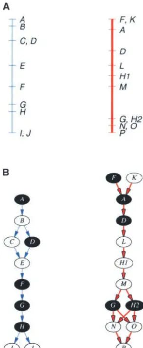
has been applied to questions of locus order on genetic, Conventionally, a map is represented by a line seg-physical, and sequence-based maps. Benzer’s (1959) ment upon which are placed the individual loci at posi-work to map point mutations in a gene has been cited tions proportional to their distance from each other. byGolumbicandShamir(1992) as one of the motiva- Figure 1A shows corresponding maps from two different tions for the study of a particular type of graph known mapping studies. (The different mapping studies are as interval graphs. Interval graphs have since been used color coded blue and red to more easily differentiate in physical mapping to solve ordering problems in yeast them. On a monochrome copy, the different studies are artificial chromosome contig assembly (Harley et al. represented by thin and thick arrows, respectively.) Fig-1996, 1999; Randall1997; Fasuloet al. 1999), radia- ure 1B shows how a map may be modeled as a graph; tion hybrid mapping (Ben-DorandChor1997;Slonim this emphasizes the order of (but not the distance
be-et al. 1997), and genomic sequence assembly (Idury tween) loci along the map. Each locus is modeled as a and Waterman 1995; Myers 1995). The problem of node, represented by an ellipse, and is connected to determining the order of genetic markers along a link- immediately adjacent loci by arrows (i.e., edges). The age group for genetic mapping may be modeled as a direction to which the arrows point is defined by some special case of the traveling salesman problem, which convention of order (e.g., from the short to the long arm is a classic problem in graph theory (LanderandGreen of the chromosome). Thus, if locusAis mapped before 1987;Liu1998, Chap. 9). These applications of graph locusB, this may be represented by a graph (A→B). theory all deal with the de novo ordering of markers A locus represents a marker mapped at a distinct within a single mapping population or set of experi- position along a map. Hence, if a single marker exhibits
ments. several polymorphisms, each of which maps to a
(1998); the same marker RG146 was used to detect the locus in both cases.
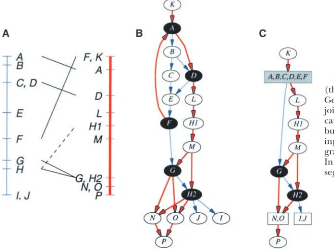
Figure 2A illustrates the problem of assigning locus equivalences across different map studies. Marker H, when used in the blue study, displayed only a single mappable polymorphism and therefore only a single locus H. Using the same marker in the red study, on the corresponding linkage group, two polymorphisms were detected and mapped and designated lociH1and H2. Matching H with H1 leads to an inconsistency in the linkage graph while matching it withH2does not. NodesHandH2are therefore designated as equivalent anchor nodes to be merged in the next step.
Merging anchor nodes:The key step in producing an integrated graph is merging the separate map graphs on the basis of their anchor nodes. Figure 2B shows the integrated graph resulting from the linkage graphs depicted in Figure 1B. The edges have been drawn in different colors to enable visual differentiation of the different mapping studies.
Intuitively, this can be accomplished by first drawing the linkage graph for one study and then iteratively adding in the connections for subsequent studies. Any appropriately labeled nodes that are already on the graph are used, with new nodes being added as neces-sary. New edges are added as in the original graph. Note that edges from the separate studies are kept distinct from each other. That is, if two studies each define (A→ B), the integrated graph will merge nodes A and B and have two edges (A→→B).
Mathematically, this operation is performed as a union Figure1.—Modeling maps as directed acyclic graphs and
of the node sets of the separate linkage graphs. How-identification of anchor nodes (thin line, blue study; thick
ever, to keep the edges representing different map stud-line, red study). (A) Corresponding maps from two different
mapping studies. (B) The respective map graphs with anchor ies distinct, only nodes are merged and not edges.
Be-nodes shaded. cause the merger is performed as a set operation, it
occurs simultaneously across all linkage graphs. There is, therefore, no bias for any particular study. At this the different studies have used some markers in com- point, the integrated graph represents a complete pic-mon, referred to asanchor markers. In a map graph, anchor ture of all of the mapping studies that comprise it; unlike markers are modeled byanchor nodes. These represent any of the four existing approaches outlined previously, equivalent loci that were mapped using the same under- our method has neither lost nor hidden any information lying marker. In Figure 2, markers A, D, F, G, and H about ambiguities and inconsistencies.
were used in both studies and are therefore designated Identifying inconsistencies: Cycles in the integrated as anchors. graph indicate an inconsistency in locus order. Intuitively, In the mapping literature, the concepts ofmarkerand consider a map that specifies the locus orderX→Ywhile
locus are often treated synonymously; indeed, locus the equivalent map from another mapping study
speci-names are usually derived from (if not identical to) fies the opposite orderY→X. The resulting integrated the corresponding marker names. However, if a single graph would show arrows that point in opposite direc-marker yields multiple mappable polymorphisms, it will tionsX ←→ Y,i.e., a cycle.
Figure2.—Production of an integrated graph (thin line, blue study; thick line, red study). (A) Genetic maps from Figure 1A with common loci joined by solid black lines. The dashed line indi-cates thatHcould have been matched withH1, but a more consistent order is produced by match-ing it toH2. (B) The corresponding integrated graph generated by merging anchor nodes. (C) Integrated graph with condensed SCC and co-segregating nodes.
of nodes and edges that connects the two nodes.) In they all come before another particular node. Hence, they may also be represented by a single condensed the red linkage graph, however, there is a pathF→A.
The two graphs are inconsistent. When the two graphs node. Similarly, nodes {I,J} cosegregate in the blue study and can therefore be represented by a single condensed are merged, this inconsistency in order is reflected as a
cycle in the integrated graph. The nodes involved in the node. However,Pcan be ordered after {N,O}. We can therefore deduce a global ordering of markers as cycle {A,B,C,D,E,F} cannot be ordered relative to each
other without yielding a contradiction (Figure 2B).
(K→{A,B,C,D,E,F}→L→H1→M→G→H2→{{I,J}, ({N,O}→P)}). The concept of a cycle is generalized as a strongly
connected component(SCC). For each pair of nodesuand Note that this string representation is similar to the notation used by MAPMAKER. Arrows define order of v within an SCC, there is a path u → v and a return
path v → u. Thus an SCC defines a cycle or several elements. If elements are unordered, they are separated by commas. Parentheses are used to group together interlocking cycles. A number of very efficient
algo-rithms are able to find the SCCs in a graph (e.g.,Cormen ordered elements; curly braces are used to group ele-ments with undefined order. Although suitable within et al.1990). The advantage of detecting inconsistencies
as SCCs is that it is as easy to detect them in integrated text for discussing relatively simple graphs or sections of graphs, this rendering quickly becomes cumbersome graphs involving three or more map studies as it is to
detect them in graphs that involve only two studies; the for more complex graphs.
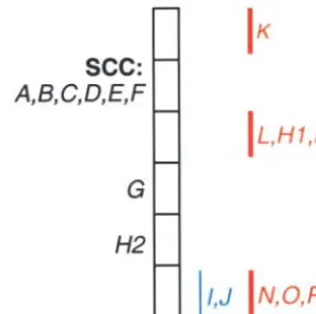
Dissecting inconsistencies:Even within an SCC, it may algorithm is affected by additional map studies only
inso-far as these studies add additional nodes to be processed. still be possible to resolve the order of certain elements, even though the SCC as a whole indicates an inconsis-Global ordering of nodes: Despite the presence of
local inconsistencies in the maps being integrated, it is tency. One way to do this is by determining which set of edges would, if removed, eliminate the cycle. Finding still possible to resolve the global order of markers that
are not involved in the inconsistency. This is accomplished the smallest such set may not always have a biological explanation, but it would be the most parsimonious in the integrated graph by “condensing” the subgraph
that comprises an SCC into a single node. Thiscondensed solution. Consider the SCC discovered previously (Fig-ure 3A). If we removed the edge (F→A), the resulting nodecan be treated as a single discrete unit within the
context of the encompassing integrated graph. graph would be acyclic (Figure 3B). We could also re-move (E → F) to break the cycle (Figure 3C). Either From Figure 2B, nodes {A,B,C,D,E,F} form an SCC
that is condensed to form the resulting graph shown in edge would be an acceptable solution.
The smallest set of edges that may be removed to Figure 2C. The condensed node can be ordered after
node Kand before nodeL. Additionally, the order of leave an acyclic graph is called theminimum feedback edge set. The problem of finding such a set is NP-complete nodes {N,O} cannot be resolved relative to each other
in the red study (i.e., they are cosegregating). These and, hence, no algorithms are known that can solve this efficiently (Garey and Johnson 1979). However, inte-nodes both have similar topology, in that they all come
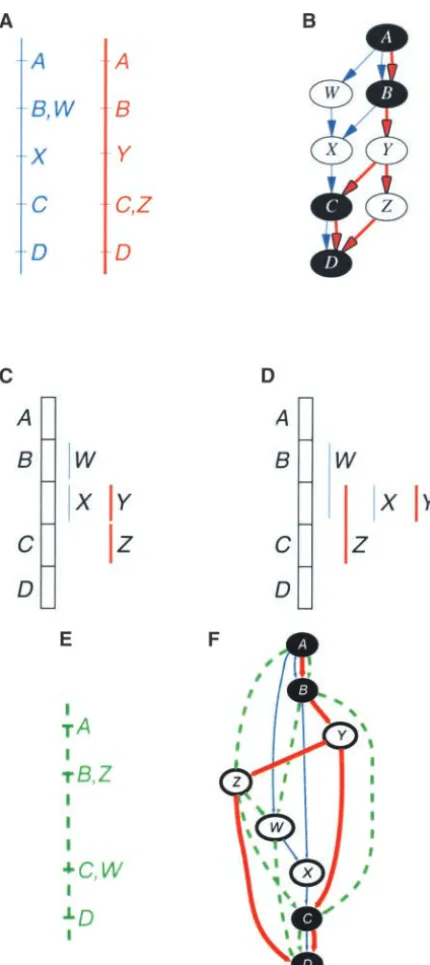
Figure 4.—Simultaneous comparison of (A) three maps Figure3.—Feedback edge sets (thin line, blue study; thick
by graph integration reveals a (B) three-way inconsistency line, red study). (A) The SCC from Figure 2B. (B) Resulting
involvingB, C, and D (thin line, blue study; thick line, red graph when (F→A) is removed. (C) Resulting graph when
study; dotted line, green study). (E→F) is removed.
blue study, cannot be ordered relative toNandO, which sparse, where each node is generally connected to a small
were mapped only in the red study. Furthermore, al-set of other nodes—those representing the preceding
though P can be definitively ordered after {N, O}, its loci and those representing subsequent loci. Further,
order relative to {I,J} is still ambiguous. an SCC generally occurs only in a limited part of the
Higher-order comparisons: The examples thus far entire integrated graph. Hence we may be able to simply
have used only two maps for integration. Multiple maps use the brute-force approach of testing every edge in
may be integrated as easily as two using the graph ap-an SCC to see whether its removal would leave ap-an acyclic
proach. Indeed, certain inconsistencies may become evi-graph. This will find all feedback sets with a single edge.
dent only when integrating three or more maps. Con-If no set has been found, then—given a sufficiently small
sider Figure 4, where three different studies mapped SCC, or enough time and computing power—this
brute-some combination of four out of five loci. Simple pair-force algorithm could be extended to find all pairs, then
wise comparisons of red to green, red to blue, and green sets of three, and so on.
to blue are not inconsistent. Only if we perform a simul-Note that there may be more than one minimum
taneous comparison of the three maps do we find that feedback edge set. In Figure 3, two sets (each composed
there is indeed an inconsistency involving all three stud-of a single edge) were found. Larger or more complex
ies. Note that none of the existing approaches to map SCCs may well have many feedback edge sets.
integration would highlight this kind of inconsistency. Identifying ambiguities: In addition to
inconsisten-Graph representation: As a data structure, the inte-cies, the graph approach may also highlight ambiguities
grated graph is the most accurate representation of the in locus order between different map studies. This is a
marker order specified by the various map studies that more subtle problem caused by insufficient
informa-comprise it. Note that it is not necessary to visualize the tion, such as when different studies use different subsets
graph to analyze it. Indeed, a major difficulty with graph of markers or when markers cosegregate on a single
visualization is that an integrated graph (indeed, any genetic map. Returning to the blue study in Figure 1A,
kind of abstract graph) may be rendered in a variety of due perhaps to lack of recombination betweenC and
ways. Two different graph representations that appear D, the two loci mapgeneticallyto the same position. This
to be visually distinct may actually describe the same set does not mean, however, that they are at the same
physi-callocation on the chromosome. Hence, a more precise of relationships. Hence, it may be difficult to compare visually two distinct graph representations to see whether statement would be that bothC and D are known to
come afterBand beforeE, but their order relative to they describe the same graph or different graphs. Graphs that are equivalent in this manner are referred to as each other is unknown. This is reflected in the blue
map graph in Figure 1B, which shows that nodesCand isomorphic. Rather than simply comparing where nodes are positioned, one must examine the edges to determine Dare both connected to the previous nodeB and the
subsequent nodeE, butCandDare not connected to whether they describe the same set of relationships. Condensed nodes:Despite its limitations, visualizing each other. The lack of a connection or path between
C and D indicates the ambiguity in their order. The a graph may still aid in understanding how nodes (i.e., loci) are ordered relative to each other. If the maps same ambiguity in ordering is true for {I,J} in the blue
study and for {F,K}, {G,H2 }, and {N,O} in the red study. being integrated have more than a moderate number of loci, their integrated graph may become visually com-In an integrated graph, the same lack of a path
be-tween nodes can indicate ambiguity in locus orderbe- plex. One way to reduce complexity without loss of infor-mation is to condense certain logically related sets of tweendifferent mapping studies. Examining Figure 2B,
Figure6.—Interval representation of the integrated graph from Figure 2B.
Figure5.—Condensed nodes (thin line, blue study; thick line, red study). (A) Integrated graph with condensed
nonan-if an integrated graph has an SCC, then it is obviously chor nodes. (B) Fully condensed integrated graph. (C) Graph
with redundant edges removed. not possible to portray the graph in linear form.
There-fore, an SCC must be treated as a single condensed node, as in Figure 2C. To further simplify the problem, that may be treated like any other node in the graph. we can also condense nonanchor nodes and remove We have already shown in Figure 2C how an SCC as redundant edges, as in the condensed graph shown in well as cosegregating markers may be condensed into Figure 5C.
a single discrete node. Certain other sets of nodes may The condensed graph intuitively suggests an interval also be condensed without altering the overall topology representation like that in Figure 6. The anchor nodes of the integrated graph. (including the SCC) are placed as intervals, in the order A series ofadjacentnodes (i.e., a contiguous series of specified by the condensed graph (SCC→ G → H 2). nodes) that are not anchors may also be condensed. Intervals representing condensed nonanchor nodes can These represent loci that were mapped in only one study then be placed relative to the anchor intervals. From and therefore add no additional information to locus the blue study, node {I,J} was ordered afterH 2, while ordering between studies. In Figure 5A, the sequential B,C, andEare already incorporated into the SCC. From nonanchor nodes (L→ H1 →M) are represented by the red study,Klies before the SCC, {L,H1,M} can be a single condensed node. Further, nodePcan also be found between the SCC andH2, and {N,O,P} can be condensed into the previously condensed {N,O} to form found afterG.
a single condensed node containing ({N,O}→P). Ambiguous orders and misleading intervals: The Figure 5B shows an even more compact graph repre- problem in constructing an interval representation is sentation, in which each condensed and nonanchor to accurately portray the ambiguities present in the inte-node has been reduced in size and labeled with the grated graph. If such an interval representation exists, number of loci represented by that node. This rendition then the graph is known as aninterval order(Fishburn has a particular advantage in that it hides the visual 1985).GolumbicandShamir(1992) indicate that de-complexity caused by markers that were mapped in only termining whether a graph is an interval order is solv-a single study, including multiple cosegregsolv-ating msolv-ark- able in polynomial time; however, the graph may not ers. It also emphasizes the order of common markers be representable at all (i.e., an integrated graph is not and highlights the inconsistent portion of the graph. necessarily an interval order).
Figure 5C shows a further simplification, in which re- Consider the two maps shown in Figure 7A. The inte-dundant edges have been hidden. These are edges that grated graph, shown in Figure 7B, tells us that an interval can be safely removed because they contribute no addi- representation would need to satisfy all of these con-tional information in terms of node ordering. straints:
Interval representation:An integrated graph carries
1. AprecedesBprecedesCprecedesD. complete information about the relative locus ordering
2.WprecedesX. of the map studies that comprise it. However, this
repre-3. YprecedesZ. sentation may become quite visually complex, making
4. XandYboth fall betweenBandC. it difficult to follow the ordering of loci. We have
ex-5. X overlaps Y (i.e., the relative order of X and Y is plored the construction of a linear representation to
unknown because there is no path betweenXandY). reduce visual complexity. Nodes are represented as
inter-6. WoverlapsB. vals, which represent the uncertainty in their position.
counterintuitive thatZcould fall beforeW, but consider that a third study that specifies the orderZ→ W (Fig-ure 7E) may be integrated without introducing an in-consistency (Figure 7F). In fact, there is no interval representation that can accurately portray all of these constraints. Only the integrated graph can represent ambiguities and inconsistencies accurately in all cases. Despite this, interval representation is sometimes useful in gaining a simplified picture of the order of nodes.
EXAMPLE
To illustrate the utility of the graph-theoretic ap-proach, we use it to analyze maps of chromosome 1 of rice (Oryza sativaL.). Several dense molecular genetic maps have been developed by different groups from diverse populations. Among these are the interspecific
O. sativa ⫻ O. longistaminata BS125/2/BS125/WLO2
population (Causseet al.1994;Wilsonet al.1999), the intersubspecific indica ⫻ japonica IR64/Azucena dou-bled-haploid population (Temnykh et al. 2001), and thejaponica⫻indicaNipponbare/Kasalath population (Harushimaet al.1998). The first two maps were devel-oped at Cornell University, mostly using simple se-quence repeat and restriction fragment length polymor-phism (RFLP) markers. They are referred to in this article as the SL01 and DH01 maps, respectively. The third was developed by the Japanese Rice Genome Proj-ect, using an independently developed set of RFLP markers. In this article, it is referred to as the JP98 map. The release of chromosome 1 sequence bySasakiet al. (2002) affords us the opportunity to test certain infer-ences generated by comparing these three genetic maps.
The total numbers of mapped markers on the SL01, DH01, and JP98 maps were 129, 91, and 289, respec-tively. Certain markers have been mapped in common between the three maps, which provides a foundation for genetic map alignment and integration. The num-ber of common (anchor) markers is relatively low, how-ever. There are 17 common markers between the SL01 Figure7.—Inaccurate interval representation (see text for
and DH01 maps, 15 between the SL01 and JP98 maps, details).
and 2 between the DH01 and JP98 maps. Among all three maps, only 2 markers were mapped in common. Figure 8 shows the three maps aligned on the basis of 8. Woverlaps Y.
anchor markers. 9. Xoverlaps Z.
Inconsistencies:The integrated graph of chromosome 10. Woverlaps Z.
Figure8.—Three genetic maps of chro-mosome 1 of rice aligned on the basis of anchor markers. Anchor markers are con-nected by cyan lines. Inconsistencies in lo-cus order between maps are indicated by red-shaded regions. Ambiguous intervals between SL01 and DH01 are indicated by a magenta-shaded region in SL01 con-nected by an arrow to the corresponding region on DH01. Ambiguous intervals be-tween SL01 and JP98 are similarly indicated by blue-shaded regions. Ambiguity between DH01 and JP98 is not indicated.
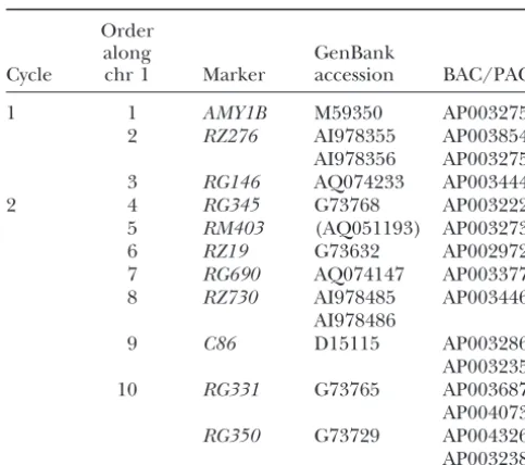
and AP003275, respectively; note that AMY1B and RM403}. Twelve minimum feedback edge sets (MFES) were RG276.Rhit the same PAC whileRG146was not identi- found, each involving removal of three edges:
fied on that PAC (Table 1).
According to the chromosome 1 sequence published by the International Rice Genome Sequencing Project, these clones are in the order AP003275→AP003444→ AP003854 (Sasakiet al.2002), indicating that the markers should be orderedAMY1B→RZ276→RG146. This is a different order from that specified by either DH01 or
C 86→RG381; RG345→RG381; RG690→RZ19
C 86→RG381; RG345→RG381; RZ19→RG690
C 86→RG381; RG381→RM403; RG690→RZ19
C 86→RG381; RG381→RM403; RZ19→RG690
C 86→RG381; RM403→RG345; RG690→RZ19
C 86→RG381; RM403→RG345; RZ19→RG690
RG331→RG350; RG381→RM403; RG690→RZ19
RG331→RG350; RG381→RM403; RZ19→RG690
RG350→C 86; RG381→RM403; RG690→RZ19
RG350→C 86; RG381→RM403; RZ19→RG690
RG381→RM403; RG381→RZ 730; RG690→RZ19
RG381→RM403; RG381→RZ 730; RZ19→RG690
SL01. BothAMY1B andRG146were mapped at a low LOD on SL01; thus this inconsistency was likely due to statistical error inherent in the genetic mapping pro-cess. Alternatively, there may be true differences in the genomes of the parental lines.
The second inconsistency involved almost the entire long
These sets were used to focus attention on intervals arm of the chromosome and contained anchors {RG690,
in-Figure9.—Integrated graph of chro-mosome 1. Locus orders specified by DH01, SL01, and JP98 are indicated by boldface red, dashed green, and blue arrows, respectively. (A) Complete inte-grated graph of chromosome 1 showing two SCCs. (B) Top portion of the inte-grated graph. This rendering is iso-morphic to the corresponding subgraph in A. The graph has been redrawn to better illustrate certain relationships. An ambiguous interval between SL01 and JP98 is indicated by a blue-shaded box. This overlaps or encompasses certain ambiguous intervals between SL01 and DH01, indicated by magenta boxes with rounded corners.
cluded the edge RZ19 → RG690, which is the order
RM403→ RG345
specified on the DH01 map with a distance of 6.5 cM
between these two loci. The other half included the RG381→ RZ730 opposing edgeRG690 →RZ19, which is the order on
RG331→ RG350
the SL01 map at 3.7 cM. Sequence forRZ19andRG690
can be found in GenBank with accessions G73632 and RG345→ RG381 AQ074147, which can be mapped to genomic BAC/
Of these nine edges, two have already been accounted PACs AP002972 and AP003377, respectively. Since the
for. Hence only seven edges with seven markers need to BAC/PACs were ordered AP002972→ AP003377, the
be examined more closely. First, the two markersRG331 loci are therefore ordered RZ19 → RG690 on the
se-andRG350appear together on the same map only on
quence-based map.
SL01. Their order, RG331 → RG350, is confirmed by To resolve the rest of the region, note that the 12
comparison to chromosome 1 sequence (Table 1). Next, MFES specified only nine edges and nine markers:
observe that the distance between RM403 and RG345 is only 1.6 cM on the SL01 map while the same two
RG381→ RM403
markers mapped in reverse order at a distance of 16
RZ19→ RG690
cM on the DH01 map. This suggests that the order of
RG690→ RZ19 these two markers may have been reversed on the SL01
map due to a low frequency of recombination in this
C 86→ RG381
region, while ordering was much clearer on the DH01 population in which recombination was high, providing
Order The magenta boxes in Figure 9B represent ambiguity
along GenBank between SL01 and DH01 in the intervalsRG246–RG532,
Cycle chr 1 Marker accession BAC/PAC RG532–RG173, andRG173–R210. Likewise, in Figure 8,
magenta-shaded intervals on SL01 point to
correspond-1 1 AMY1B M59350 AP003275
2 RZ276 AI978355 AP003854 ing intervals on DH01. Note how the magenta- and
blue-AI978356 AP003275 shaded intervals overlap each other. This shows how
3 RG146 AQ074233 AP003444 ambiguities may overlap, depending on the pair of
com-2 4 RG345 G73768 AP003222 parisons being made. These ambiguous intervals may
5 RM403 (AQ051193) AP003273
be considered to define a set of bins within which locus
6 RZ19 G73632 AP002972
order is only partially known, but the boundaries of the
7 RG690 AQ074147 AP003377
bins depend on which set of comparisons is being made.
8 RZ730 AI978485 AP003446
AI978486 In Figure 8, lines connecting anchor loci may
them-9 C86 D15115 AP003286 selves indicate ambiguity, if loci cosegregate to that
posi-AP003235 tion. For example, on chromosome 1,RG246andRZ288
10 RG331 G73765 AP003687 cosegregate in SL01, but DH01 mapped only RG246
AP004073
and JP98 mapped onlyRZ288. This is reflected in the
RG350 G73729 AP004326
integrated graph, in which there is no path between AP003238
the nodes representingRG246 andRZ288. Hence, no The corresponding GenBank accession(s) for each marker conclusion can be drawn as to the relative order of are given along with the significant hit for that sequence to
these two loci since there is no evidence (due to lack of genomic BAC/PAC sequence. Chr, chromosome.
recombination, small population size, double crossover, missing data, etc.) to prefer one order over the other. less chance of statistical error. Comparison to genomic
sequence confirmed that the order should indeed be
DISCUSSION
RG345 → RM403. Similarly, the sequence-based map
confirms the locus orderC86→RG350as given by the An implicit assumption behind the notion of an inte-grated map is the view that, for a species as a whole, SL01 map, rather than the reverse order shown on JP98.
The remaining edges all involved RG381. Unfortu- there is one correct order of markers. Under this as-sumption, the data from individual mapping studies— nately, sequence for this marker is not available.
How-ever, note that marker RG381 was mapped on SL01 using different crosses and different sets of markers— represent different samplings of the species map. Thus, as locus RG381X. This indicates that this marker was
observed to have multiple copies on the basis of hybrid- the objective of map integration is to combine individual primary maps into a single integrated species map. The ization signal on Southern blots, only one of which
was mapped (Causseet al. 1994;Wilson et al. 1999). four approaches to map integration currently in use have as their goal to generate a simplified resolution of Reexamination of the existing hybridization filters
indi-cates that marker RG381does indeed exhibit multiple the inconsistencies and ambiguities that exist in the data. Presentation of a single integrated map tends to bands and is likely to map to more than one position
in the rice genome (S.Harrington, personal commu- obscure these anomalies; our graph approach, on the other hand, highlights them. It is of interest to compare nication). It appears, therefore, that one copy ofRG381
may have been mapped to position 112.35 cM on SL01 the way these different approaches handle inconsisten-cies and ambiguities.
and another copy to position 117.1 cM on DH01.
Ambiguities:Examination of the integrated graph for One conceptualization of consensus mapping is that marker positions may be averaged across the different pairs of nodes that havenopath between them detects
ambiguity. Figure 9B shows the integrated graph for the mapping studies being integrated. This is the view taken directly by the variousad hocvisual approaches to map top portion of chromosome 1. Note that within the
blue-shaded region is a node with the label “JP98-6”; this integration. The visual approach is arguably the most flexible of the four approaches, since access to the raw represents the loci that were mapped only on JP98
within the interval delineated byG359andR210. Note marker segregation data is not required. This was the method of choice for the creation of the wheat consen-further that no path exists from JP98-6 to any of the
other nodes (SL01-7,RG532, SL01-8,RG173, and SL01- sus map, for instance, where the problem involved bringing together maps from the three different ge-9) within the blue region, all of which were mapped
allo-hexaploid species (Nelsonet al.1995a,b,c;Van Deynze estimates for recombination fractions are then used to compute new expected values and the process is re-et al.1995; Marinoet al.1996). Since construction of
the consensus map involved integration across three peated until the likelihood converges into a maximum. MAPMAKER uses a hidden Markov chain model de-homeologous groups of chromosomes that do not
re-combine with each other, this precluded the use of scribed byLanderandGreen(1987) to simultaneously compute the expected number of recombinant meioses existing mapping software. The disadvantage of visual
interpolation is that it is highly subjective and hence and the maximum-likelihood recombination fractions. The models to estimate the recombination fractions not wholly reproducible. It is also difficult to visually
integrate more than two or three maps at a time. and maximum likelihood are dependent on population size and structure. Because of this, one cannot use MAP-The GDB (1999) approach prescribes a heuristic
algo-rithm, in which a specific map is designated as the stan- MAKER or similar software to create an integrated map from an arbitrary set of mapping populations. However, dard map. The coordinate system of a second map is
then projected onto the standard map. The resulting map integration is possible if the populations are of similar size and identical structure. The pooled map for “comprehensive” map is then used as the basis for
incor-porating the next map. This process is iterated until all maize developed by Beavis and Grant (1991) used data from four different maize populations with similar maps have been incorporated into the comprehensive
map. It is more objective than the visual approach and numbers of individuals. Essentially, the individual popu-lations were treated as different replications of a single can be used to integrate multiple maps of different
types. Although access to the raw data is not necessary, map study. For the most part, however, an arbitrary set of mapping studies will differ in population size, it requires that the map distances between markers be
known. Most importantly, the final comprehensive map structure, and resolution (i.e., number of markers), ren-dering invalid the assumptions of standard mapping is dependent on the order in which the primary maps
are incorporated. software such as MAPMAKER.
As an alternative to software such as MAPMAKER, Despite progress in physical and sequence-based
map-ping, genetic linkage maps are often the only type of JoinMap was designed to allow integration of genetic maps from disparate populations. Pairwise recombina-map available for many species. Genetic recombina-maps continue
to be a valuable tool for genomic research. They are tion frequencies are calculated as well as LOD scores for those pairs that are available in the entire data set. often used to guide the assembly of physical and
se-quence-based maps. Genetic mapping monitors the re- Beginning with the most informative pair of markers, JoinMap iteratively builds up the map by adding a new combinatorial process, allowing researchers to
deter-mine how genes are inherited in relationship to other marker on the basis of LOD score. The best-fitting posi-tion of this new marker is determined without changing genes in the genome. This is useful, for instance, when
studying coinheritance or coregulation of linked genes, the order of markers that were placed earlier. Periodi-cally, the locus orders are reshuffled so that the best-fit investigating the evolutionary significance of conserved
chromosomal segments (homeologous regions) be- order for the entire map can be found. JoinMap adjusts for the differences in population size and structure by tween species, or designing a plant or animal breeding
strategy. assigning different weights when estimating map distances
(Stam 1993). However, this still does not account for When all the maps to be integrated are genetic maps
and the raw segregation data are available, it becomes the fact that different sets of parentals have differentially nonlinear recombination rates along the length of the possible to plug these data into standard mapping
soft-ware such as MAPMAKER. MAPMAKER first estimates chromosome. Further, crossovers occur nonrandomly in the genome. Observed recombination frequency not the most likely order of loci on the basis of two-point,
three-point, and multipoint recombination values. Then only varies with distance from the centromere, but also varies due to crossover interference, the presence of it computes a genetic map on the basis of the estimated
locus order. With complete data, one can simply count recombinatorial “hot spots” and “cold spots,”e.g., genes that change the rate of recombination either in cisor the number of meiotic recombinations that occurred
between loci, adjust that data to take account of the in trans(Muller1916), and nonrandom gamete elimi-nation resulting from both genetic and environmental probability of double-crossover events, and compute
re-combination fractions (and hence genetic distance). causes.
Different maps produced by different studies are as-To handle missing data, MAPMAKER uses an iterative
procedure to estimate recombination fractions. From sumed to sample the same underlying physical order of markers. However, there will invariably be differences an initial guess for the recombination fractions, the
expected number of recombinant and nonrecombinant in marker order among the different studies. Resolving these inconsistencies prior to the construction of the meioses in each interval for the complete data is
com-puted as if the guess were actually correct. From this consensus map generally requires an investment in addi-tional laboratory work and can be very labor intensive expected value, the maximum-likelihood estimate for
among individuals of the same species due to
duplica-Benzer, S., 1959 On the topology of the genetic fine structure. Proc. tions, translocations, inversions, or movement of trans- Natl. Acad. Sci. USA45:1607–1620.
posable elements as has been recently demonstrated by Causse, M. A., T. M. Fulton, Y. G. Cho, S. N. Ahn, J. Chunwonseet al., 1994 Saturated molecular map of the rice genome based on FuandDooner(2002).
an interspecific backcross population. Genetics138:1251–1274.
Cho, Y. G., S. R. Mccouch, M. Kuiper, M.-R. Kang, J. Potet al., 1998 Integrated map of AFLP, SSLP and RFLP markers using a recombinant inbred population of rice (Oryza sativaL.). Theor.
CONCLUSION Appl. Genet.97:370–380.
Cormen, T. H., C. E. LeisersonandR. L. Rivest, 1990 Introduction
We have taken a novel approach to map integration
to Algorithms. MIT Press, Cambridge, MA.
by modeling maps as graphs. Map integration and analy- Fasulo, D., T.Jiang, R. M.Karp, R. J.Settergrenand E.Thayer, 1999 An algorithmic approach to multiple complete digest map-sis are performed on these graphs and include the
fol-ping. J. Comput. Biol.6:187–207. lowing steps:
Fishburn, P. C., 1985 Interval Orders and Interval Graphs: A Study of Partially Ordered Sets. John Wiley & Sons, New York.
1. Identifying and merging anchor nodes Fu, H., andH. K. Dooner, 2002 Intraspecific violation of genetic 2. identifying inconsistencies colinearity and its implications in maize. Proc. Natl. Acad. Sci.
USA99:9573–9578. 3. global ordering of nodes
Garey, M. R., andD. S. Johnson, 1979 Computers and Intractability:
4. dissecting inconsistencies A Guide to the Theory of NP-Completeness. W. H. Freeman, New York. 5. identifying ambiguities. GDB, 1999 GDB comprehensive map construction (http://www.gdb.
org/).
Golumbic, M. C., andR. Shamir, 1992 Complexity and algorithms Although an integrated graph may not be amenable
for reasoning about time: a graph-theoretic approach. J. ACM to direct inspection, it can be used as a data structure to
40:1108–1133.
drive analysis in an objective and reproducible manner. Harley, E., A. J. BonnerandN. Goodman, 1996 Good maps are straight, pp. 88–97 inProceedings, Fourth International Conference
The algorithms described in this article are very efficient
on Intelligent Systems for Molecular Biology (ISMB), edited byD. J.
and relatively easy to implement.
States, P. Agarwal, T. Gaasterland, L. HunterandR. Smith. This approach to map integration allows for compari- AAAI Press, Washington University, St. Louis. (ftp://ftp.cs.toronto. sons purely on the basis of marker order and does not edu/%2Fcs/ftp/pub/bonner/papers/genome.mapping/).
Harley, E., A. BonnerandN. Goodman, 1999 Revealing hidden require access to the raw mapping data or information
interval graph structure in STS-content data. Bioinformatics15: about distances between markers. Furthermore, it can 278–285.
be used to integrate maps of different types, such as Harushima, Y., M. Yano, A. Shomura, M. Sato, T. Shimanoet al., 1998 A high-density rice genetic linkage map with 2275 markers genetic, physical, or sequence based. Each linkage
using a single F2population. Genetics148:479–494.
graph, in essence, is a statement about the order of Idury, R. M., andM. S. Waterman, 1995 A new algorithm for DNA markers derived for that linkage group from that partic- sequence assembly. J. Comput. Biol.2:291–306.
Kianian, S. F., andC. F. Quiros, 1992 Generation of aBrassica oleracea
ular mapping study. Map integration using these
di-composite RFLP map: linkage arrangements among various popula-rected graphs allows us to reason directly about marker tions and evolutionary implications. Theor. Appl. Genet.84:544– order and more easily determine both similarities and 554.
Lander, E. S., andP. Green, 1987 Construction of multilocus genetic differences between distinct maps from different
stud-linkage maps in humans. Proc. Natl. Acad. Sci. USA84:2363–2367. ies. When used directly, the resulting integrated graph
Lander, E. S., P. Green, J. Abrahamson, A. Barlow, M. J. Daly
is a faithful representation of the marker orders of its et al., 1987 MAPMAKER: an interactive computer package for constructing primary genetic linkage maps of experimental and component maps, including all of their ambiguities and
natural populations. Genomics1:174–181. inconsistencies. Knowledge of where these irregularities
Lincoln, S. E., M. J. DalyandE. S. Lander, 1993 Constructing Genetic
occur can help to motivate additional research into in- Linkage Maps with MAPMAKER/EXP Version 3.0: A Tutorial and Refer-vestigating the biological reasons, if any, behind the ence Manual. Whitehead Institute, Cambridge, MA (http://www.
broad.mit.edu/ftp/distribution/software/mapmaker3/). inconsistencies or to better choose markers to resolve
Liu, B. H., 1998 Statistical Genomics: Linkage, Mapping, and QTL
Analy-ambiguities. sis. CRC Press, Boca Raton, FL.
Marino, C. L., J. C. Nelson, Y. H. Lu, M. E. Sorrells, P. Leroyet
We acknowledge Golan Yona, Pankaj Jaiswal, and two anonymous
al., 1996 Molecular genetic maps of the group 6 chromosomes reviewers for their invaluable comments and suggestions. We also
of hexaploid wheat (Triticum aestivumL. em. Thell.). Genome thank Lois Swales for her help in formatting and submitting. The
39:359–366. software package Graphviz, used to render the graphs in this article,
Muller, J., 1916 The mechanism of crossing over. Am. Nat.50: is available for download at http://www.graphviz.org. This work was 193–207.
funded in part by the U.S. Department of Agriculture-Agricultural Myers, E. W., 1995 Toward simplifying and accurately formulating Research Service (USDA-ARS) specific cooperative agreements 58- fragment assembly. J. Comput. Biol.2:275–290.
and rearrangements in homoeologous groups 4, 5, and 7. Genet- the Calculation of Genetic Linkage Maps. CPRO-DLO, Wageningen, The Netherlands.
ics141:721–731.
Nelson, J. C., A. E. Van Deynze, E. Autrique, M. E. Sorrells, Y. H. Tani, N., T. Takahashi, H. Iwata, Y. Mukai, T. Ujino-Iharaet al., 2003 A consensus linkage map for sugi (Cryptomeria japonica)
Luet al., 1995b Molecular mapping of wheat: homoeologous
group 2. Genome38:516–524. from two pedigrees, based on microsatellites and expressed se-quence tags. Genetics165:1551–1568.
Nelson, J. C., A. E. Van Deynze, E. Autrique, M. E. Sorrells, Y. H.
Luet al., 1995c Molecular mapping of wheat: homoeologous Temnykh, S., W. D. Park, N. Ayres, S. Cartinhour, N. Haucket al., 2000 Mapping and genome organization of microsatellite group 3. Genome38:525–533.
Randall, J. R., 1997 Using interval graphs for solving map assembly sequences in rice (Oryza sativa L.). Theor. Appl. Genet. 100: 697–712.
problems. Master’s Thesis, Department of Computer Science,
University of Toronto, Toronto, Ontario, Canada (ftp://ftp.cs. Temnykh, S., G. Declerck, A. Lukashova, L. Lipovich, S. Cartin-houret al., 2001 Computational and experimental analysis of toronto.edu/pub/bonner/papers/genome.mapping/).
Sasaki, T., T. Matsumoto, K. Yamamoto, K. Sakata, T. Babaet al., microsatellites in rice (Oryza sativaL.): frequency, length varia-tion, transposon associations, and genetic marker potential. Ge-2002 The genome sequence and structure of rice chromosome
1. Nature420:312–316. nome Res.11:1441–1452.
Sewell, M. M., B. K. ShermanandD. B. Neale, 1999 A consensus Van Deynze, A. E., J. Dubcovsky, K. S. Gill, J. C. Nelson, M. E.
map for loblolly pine (Pinus taedaL.) I: construction and integra- Sorrellset al., 1995 Molecular-genetic maps for group 1 chro-tion of individual linkage maps from two outbred three-genera- mosomes of Triticeae species and their relation to chromosomes tion progenies. Genetics151:321–330. in rice and oat. Genome38:45–59.
Slonim, D., L. Kruglyak, L. SteinandE. Lander, 1997 Building Wilson, W. A., S. E. Harrington, W. L. Woodman, M. Lee, M. E.
human genome maps with radiation hybrids. J. Comput. Biol.4: Sorrellset al., 1999 Inferences on the genome structure of
487–504. progenitor maize through comparative analysis of rice, maize
Stam, P., 1993 Construction of integrated genetic linkage maps by and the domesticated Panicoids. Genetics153:453–473. means of a new computer package: JoinMap. Plant J.3:739–744.