MIMO Beamforming With Mutual Coupling, Limited Feedback and Coordination

(1)

DONG, YUHAN. MIMO Beamforming with Mutual Coupling, Limited Feedback and Coordination. (Under the direction of Dr. Brian L. Hughes).

Multi-input, multi-output (MIMO) techniques use multiple antennas at both the transmitter and receiver to improve the performance of wireless communications systems over multipath fading channels. In recent years, MIMO techniques that em-ploy transmit beamforming have been adopted in several new and emerging standards for situations where channel state knowledge is available at the transmitter. Most existing studies of MIMO beamforming assume that perfect channel knowledge is available at both the transmitter and receiver, and that the antenna elements in both the transmit and receive arrays are spaced sufficiently far apart so as to be essentially uncoupled. In practice, however, constraints on the physical size of antenna arrays may require elements to be spaced close together, leading to antenna coupling and signal correlation. The capacity of the feedback link from the receiver to the trans-mitter may also be limited, so that channel knowledge is necessarily imperfect at the transmitter. These challenges become all the more difficult in multiuser scenarios, when efficient coordination among several transmitters is required.

(2)

(3)

Yuhan Dong

A dissertation submitted to the Graduate Faculty of North Carolina State University

in partial fullfillment of the requirements for the Degree of

Doctor of Philosophy

Electrical Engineering

Raleigh, North Carolina 2009

APPROVED BY:

Dr. Mihail L. Sichitiu Dr. Kazufumi Ito

(4)

DEDICATION

(5)

BIOGRAPHY

(6)

ACKNOWLEDGMENTS

First and foremost, I would like to express my deepest gratitude to my advisor, Dr. Brian L. Hughes, for his guidance and continuous support throughout my PhD study. I have benefited tremendously from his wisdom, vision, technical insight, illuminating instruction, professionalism and assiduous work. He will be a truly inspiring role model for my future career.

I am grateful to the professors serving in my PhD committee: Dr. J. Keith Townsend, Dr. Mihail L. Sichitiu and Dr. Kazufumi Ito for their valuable comments and feedback. I would like to extend my sincere thanks to Dr. Gianluca Lazzi, who served as my former committee member, and is co-author of some of my papers. My gratitude is also given to Dr. Huaiyu Dai who provided useful knowledge in the general area of wireless communications in the courses he taught.

I am thankful to all colleagues from Wireless Systems Engineering (WiSE) lab for making a friendly and fruitful research environment. Carlo Domizioli and Pawandeep Singh have always been great partners for enlightening discussions. I would like to thank all my friends, here at Raleigh and elsewhere, for making my life enjoyable.

(7)

LIST OF TABLES

Table 4.1 Grassmannian codebook for N = 2, B = 3 andK = 8 . . . 62

Table 4.2 Llyod (vector quantization) codebook for N = 2, B = 3 and K = 8 . . 63

Table 4.3 IEEE 802.16e-2005 codebook for N = 2, B = 3 andK = 8 . . . 63

(11)

LIST OF FIGURES

Figure 2.1 A channel model for N ×M MIMO systems.. . . 13

Figure 2.2 AN ×M SU-MIMO system using beamforming and combining. . . 16

Figure 2.3 Outage probability of N ×M SU-MIMO MRC systems with i.i.d. Rayleigh fading. . . 21

Figure 2.4 Outage probability of 2×2 SU-MIMO MRC systems with transmitter correlation. . . 22

Figure 2.5 Outage probability of N×M SU-MIMO MRC systems with limited feedback and i.i.d. Rayleigh fading. . . 23

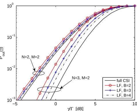
Figure 2.6 Outage probability of N×M SU-MIMO MRC systems with limited feedback B = 3 and correlated Rayleigh fading |ρ|2 _{= 0.8. . . 24}

Figure 2.7 A MIMO broadcast channel with coordinated beamforming.. . . 27

Figure 2.8 Sum-rates vs. SNR for N = 2, M = 2 or 4 with perfect CSI.. . . 32

Figure 2.9 Sum-rates vs. SNR for various N and M with perfect CSI. . . 33

Figure 2.10 Sum-rates vs. SNR for N = 2, M = 2 or 4 with limited feedback.. . . 34

Figure 3.1 Circuit model of a transmit array with mutual coupling. . . 38

Figure 3.2 Outage probabilities vs. normalized SNR with N = 2, M = 1 or 2 and spacing d= 0.3λ for three different power measures. . . 49

Figure 3.3 Magnitude of correlation coefficients vs. antenna spacingd/λ. . . 50

Figure 3.4 Outage probabilities vs. antenna spacings d/λ with N = 2, M = 2 at two outage level for three different power measures. . . 51

(12)

Figure 4.1 Outage probabilities vs. antenna spacings d/λ for N =M = 2 SU-MIMO MRC system with different feedback scenarios and power measures. 61

Figure 4.2 Outage probabilities for codebooks generated by three methods with power measure P3, B = 3 andd = 0.3λ. . . 62

Figure 4.3 Outage probabilities for codebooks W1 and W3 with power measure

P3,B = 2 and d= 0.2λ. . . 64

Figure 4.4 A N×M SU-MIMO MRC system in the presence of channel estima-tion error. . . 66

Figure 4.5 Outage probabilities vs. normalizedSNR withN =M = 2,d = 0.2λ, Pp/N0 = 10 dB and L= 2 for different power measures. . . 71

Figure 4.6 Diversity gain vs. antenna spacing d/λ for N = M = 2 SU-MIMO MRC system with power measure P3, L= 2 and Pp/N0 = 10 dB.. . . 72

Figure 4.7 Diversity gain vs. number of pilot symbols per transmission block (L) d/λ for N = M = 2 SU-MIMO MRC system with power measure P3,

d= 0.2λ,Pp/N0 = 10 dB and multiport matching. . . 73

Figure 4.8 Diversity gain vs. pilot SNR Pp/N0 for N =M = 2 SU-MIMO MRC

system with power measure P3, d= 0.2λ,L= 2 and multiport matching.. . . 74

Figure 5.1 Circuit model of anM-antenna receiver with mutual coupling. . . 85 Figure 5.2 Sum rate vs. SNR with N =M = 2 andd= 0.1λ.. . . 94 Figure 5.3 Sum-rate for multiport matching vs. SNR with N = 2, M = 2 or 4

and d= 0.2λ. . . 95 Figure 5.4 Sum-rate vs. antenna spacing with N = 2, M = 4 and different

feedback scenarios.. . . 96

Figure 5.5 Outage probability vs. normalizedSNRwithN =M = 2 for different feedback scenarios.. . . 97

Figure 5.6 Diversity gain vs. antenna spacing with N = M = 2 for different feedback scenarios and noise sources.. . . 98

(13)

users. . . 103

Figure 6.2 Achievable average rate region with SNR=15 dB.. . . 118

Figure 6.3 Achievable average sum-rate vs. SNR. . . 120

Figure 6.4 Achievable average sum-rate vs. (a) number of Tx antennas with M = 3 (b) number of Rx antennas with N = 3 for SNR = 15 dB. . . 121 Figure 6.5 Achievable average sum-rate vs. parameter s with N =M = 3 and

SNR = 15 dB. . . 123

(14)

Chapter 1 Introduction

1.1 Motivation

Over the past few decades, the need for reliable, high data-rate, wireless com-munications has dramatically increased due to the growing demand for broadband mobile access to the Internet. In recent years, a wide variety of transmission schemes have been proposed that use multiple antennas at the transmitter and receiver to improve the performance of wireless systems. These schemes are collectively known as multiple-input multiple-output (MIMO) techniques.

(15)

antennas. These pioneering works predicted that MIMO techniques can achieve large spectral efficiencies, which ignited much interest in this area [40]. Over the past decade, MIMO communication techniques have been adopted in new standards for wireless local area networks (IEEE 802.11n [47]), metropolitan area networks (e.g. IEEE 802.16e [48] and 802.16m1_{), and cellular telephony (W-CDMA [44], HSPA [45]}

and LTE2 _[1]).

When channel knowledge is available at both the transmitter and receiver, beamforming techniques are a relatively simple and effective way to exploit the di-versity benefits of the MIMO channel. These techniques seek to transmit data along the dominant eigenmodes of the MIMO channel. Single-user MIMO beamforming was first considered by Lo [62]. Later, Tse et al. [90] and Dighe et al. [24] opti-mized MIMO beamformer design by using maximum-ratio transmission (MRT) and maximum-ratio combining (MRC). Kang and Alouini [55] evaluated the outage prob-ability and ergodic capacity of this optimal MIMO beamforming scheme. MIMO beamforming has also been considered for multiuser scenarios to improve the ca-pacity and reliability. Some specific MIMO beamforming techniques that use trans-mit/receive coordination to eliminate multiuser interference and improve the sum-rate are presented in [33], [97] and [14].

The ability of MIMO beamforming to adapt to changing fading conditions make it a promising technique to mitigate fading and enhance the performance over 1_{IEEE 802.11n and IEEE 802.16e modify the physical (PHY) and medium access control (MAC)}

layers of Wi-Fi (IEEE 802.11) and WiMAX (IEEE 802.16), respectively, to provide higher through-put using OFDM and MIMO technologies. IEEE 802.16m is the latest version of 802.16e and still in progress.

2_{W-CDMA defines the air interface for UMTS which, together with WiMAX, are the members}

(16)

slowly-varying channels. For this reason, MIMO beamforming has been adopted as an optional advanced transmission strategy in the wireless cellular standards mentioned earlier. Most existing studies of MIMO beamforming, however, assume that perfect channel knowledge is available at both the transmitter and receiver, and that the antenna elements in both the transmit and receive arrays are spaced sufficiently far apart so as to be essentially uncoupled. In practice, however, constraints on the physical size of antenna arrays may require elements to be spaced close together, leading to antenna coupling and signal correlation. The capacity of the feedback link from the receiver to the transmitter may also be limited, so that channel knowledge is necessarily imperfect at the transmitter. These challenges become all the more difficult in multiuser scenarios, when efficient coordination among several transmitters is required.

(17)

1.1.1 Mutual Coupling in Compact Antenna Arrays

An antenna is a transducer designed to convert electromagnetic waves into electrical currents and vice versa. However, when antenna elements are placed in close proximity, a current in one antenna will induce voltages across its neighbors [22]. This phenomenon is called mutual coupling.

Many compact wireless transceivers, such as cellular telephones and wireless LAN cards, are severely constrained in physical size. When MIMO antennas are brought close together, the electric fields detected by different elements become cor-related, the radiation patterns of each element may become distorted, mutual coupling occurs between the antennas, and power may radiated or captured less efficiently. It is therefore important to determine how close the elements of an array may be placed and still enjoy the benefits of MIMO beamforming.

When the receive antennas are coupled due to the small inter-element spacing, the noise from each receive chain may no longer be spatially white [71], [25]. Moreover, the statistics of the signal and noise will depend in general on detailed aspects of the receiver design. To optimize performance in such scenarios, it is necessary to develop realistic models of RF front-ends with coupled antenna arrays as well as new MIMO beamforming techniques that exploit these models to improve the performance.

1.1.2 Channel State Information

(18)

phenomenon is called multipath fading. When fading is frequency-nonselective, the impact of fading on the transmitted signal in a single-antenna system can be repre-sented by thefading path gain,a complex number that reflects the change in amplitude and phase of the received signal due to fading. In a MIMO channel, fading conditions may be different between each pair of transmit and receive elements, so the current

channel state is represented by a matrix H which consists of the fading path gains between each pair of transmit and receive elements.

In a MIMO beamforming system, channel state information (CSI) allows the transmitter and receiver to communicate data along the dominant eigenmode of the MIMO channel, thereby mitigating the damaging effects of fading and maximizing the output signal-to-noise ratio (SNR) of the channel. By the dominant eigenmode, we mean the singular vector of the channel state matrix H that corresponds to the largest singular value, based on the singular-value decomposition (SVD).

(19)

Perfect CSI at the transmitter can also be difficult to achieve when the capacity of the feedback link is low. One approach to performing MIMO beamforming in the presence of this impairment is to employ limited feedback (also known as finite-rate feedback) techniques [65], [98], [14]. Limited feedback techniques can significantly reduce the required capacity of the feedback link by transmitting only quantized or compressed versions of the CSI or beamforming vectors. This area of research has been very active recently due to its relevance to implementing MIMO beamforming techniques in practical settings, such as WiMAX and LTE.

1.1.3 Coordination and Interference Mitigation

For single-user MIMO (SU-MIMO) scenarios, such as point-to-point commu-nication links, MIMO beamforming can improve system reliability and maximize the output SNR over fading multipath channels. In the literature, optimal SU-MIMO beamforming is also known as MIMO maximal ratio combining (MRC) [55], [103]. In multiuser MIMO (MU-MIMO) scenarios, such as the MIMO broadcast channel (BC),3 _{MIMO beamforming techniques can also can be used to increase the number}

of users supported by the system, or to increase overall throughput.

When CSI is available at the transmitter, it is well known that the sum-capacity of the MIMO BC can be achieved by dirty-paper coding (DPC). However, DPC is difficult to implement in practice due to its high complexity [11], [94]. A simpler suboptimal method of sharing the MIMO broadcast channel is linear MIMO 3_{In a MU-MIMO broadcast system, the base station communicates with multiple mobile users,}

(20)

beamforming [20], [77]. In linear MIMO beamforming, the data symbols intended for each mobile receiver are modulated onto distinct beamforming vectors at the transmit-ter. The mobiles then separate these symbols by applying distinct linear combiners at the receiver. Since the design of these beamforming vectors and combiners generally requires coordination among the users, this type of linear beamforming is also called

coordinated beamforming (CBF) [14]. Most existing studies of CBF have considered the case of symmetric rates and uncoupled antennas. It is natural to ask how these techniques generalize to the asymmetric rate situations, and how the performance of these techniques is affected by the presence of antenna mutual coupling.

1.2 Contributions

As noted earlier, this dissertation considers the analysis and design of MIMO beamforming techniques with antenna mutual coupling, limited feedback and mul-tiuser coordination. The main contributions may be summarized as follows.

(21)

the impact of SNR and the length of pilot symbols is also addressed.

We then assume perfect channel estimation at the receiver and consider the design of finite-rate codebooks of possible beamforming vectors for three input power metrics. The receiver, who has full CSI, can then select the vector in the codebook that maximizes the output SNR and communicate the index of this vector to the transmitter via the feedback channel. The performance of limited feedback and its dependence on matching, coupling and number of feedback bits is evaluated through numerical examples. We also analyze the performance degradation for actual system when codebooks are mismatched.

Coordinated Beamforming with Mutual Coupling: Second, we consider the impact of receiver correlation, antenna coupling, matching and noise on the perfor-mance of downlink MU-MIMO coordinated beamforming systems. We first present a new coordinated beamforming technique for two receivers that is suitable for MIMO broadcast channels with signal and noise correlation at the receiver. We then ap-ply this technique to the specific type of signal and noise correlation that occurs in the presence of receiver mutual coupling by introducing a more realistic model for a multi-antenna receiver front-end. Numerical examples demonstrate how different noise sources and matching networks may impact performance in different ways. We also consider the design and performance of limited feedback techniques for coordi-nated beamforming systems and how performance is affected by receiver coupling, correlation, matching networks and noise.

(22)

symmet-ric methods for coordinated beamforming for two receivers and the MIMO broad-cast channel. By changing the design order of the transmit beamforming vectors and receive combining vectors, we develop a newsymmetric coordinated beamforming (SCBF)scheme that is linear and non-iterative. We then relax the symmetry restric-tion and propose a new asymmetric coordinated beamforming (ACBF) method. In this method, the first user employs single-user MIMO MRC, while the second user attempts to maximize his rate of transmission subject to zero-interference constraints. Finally, we consider the maximization of sum-rate over all these coordinated beamforming strategies. We propose a parameterized asymmetric coordinated beam-forming (P-ACBF) method that achieves a better tradeoff between the rates of the two users than existing methods. Numerical examples illustrate the advantage of in-troducing time-division policy into ACBF and P-ACBF, respectively, by changing the priorities of two users. A simple upper bound of the sum-rate is derived to facilitate the comparison of performance.

1.3 Outline

(23)

(24)

Chapter 2 MIMO Beamforming over Rayleigh

Fading Channels

In wireless communications, signals are transmitted through radio propaga-tion channel which determines crucially the characteristics of the entire MIMO sys-tem [75]. There are a variety of different approaches used for modeling the MIMO wireless channel to capture the realistic properties or facilitate spatial-temporal signal processing.

(25)

zero-interference constraints.

Both the MIMO beamforming strategies, i.e. SU-MIMO MRC and downlink MU-MIMO CBF, are close-loop technique and require channel state information at transmitter. In some one-way communication systems, CSI can be feed back from the receiver to the transmitter via feedback link, i.e. control channel, which is practically constrained in capacity. The effective approaches to implement limited feedback are addressed in the last section of this chapter.

2.1 MIMO Channel Model

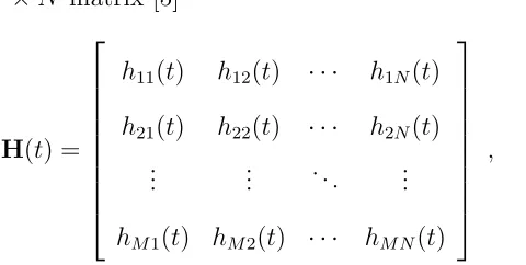
In this section, we present a MIMO channel model to understand the nature of MIMO radio channels. Consider a system employedN antennas at the transmitter and M antennas at the receiver, denoted as N ×M MIMO system and shown in Figure 2.1. In a rich scattering environment with a delay spread that is small com-pared to the inverse signal bandwidth1_{, a linear time-variant MIMO channel may be}

represented as an M ×N matrix [5]

H(t) = 

        

h11(t) h12(t) · · · h1N(t)

h21(t) h22(t) · · · h2N(t)

... ... . .. ... hM1(t) hM2(t) · · · hM N(t)



        

, (2.1)

where hmn(t) denotes the time-variant impulse response between the m-th receive

(26)

instant, we denote each individual fading path gain and channel matrix ashmnandH,

respectively. Therefore, the discrete-time input-output relation over a symbol period can be expressed in a matrix form as

r=Hx+n , (2.2)

where x is the complex baseband transmitted signal vector, r is the received sig-nal vector, and n represents additive Gaussian noise with zero-mean and covariance Rn = E

£

nnH¤_{, here} _E_[_·_{] is the expectation. We denoted the noise distribution by}

n ∼ CN(0,Rn). A reasonable model for the noise is additive white Gaussian noise

(AWGN) and therefore the covariance matrix is Rn = N0I where N₂0 is the power

spectral density of the noise in single branch and I is the identity matrix. The total transmit power isP = tr¡E£xxH¤¢_{where tr(}_·_{) is the trace and superscript}_H_denotes

conjugate-transpose.

. .

.

. .

.

1

x

N

x

11

h

MN

h

1

. .

.

Figure 2.1: A channel model for N ×M MIMO systems.

(27)

hmn ∼ CN(0,1). Since the amplitudes |hmn| are Rayleigh-distributed random

vari-ables, the multipath fading is also referred to as Rayleigh fading2_{. Then the}

chan-nel matrix H can be fully represented by a zero-mean multivariate complex normal (MCN) distribution and completely characterized by the covariance matrix R with covariance matrix R

R=E£vec(H)vec(H)H¤ _, _(2.3)

where vec(A) denotes the vectorization of the matrix A by stacking the columns of A into a single column vector. We denote this distribution by H ∼ CN(0,R). The spatial correlationof the MIMO channel can be completely characterized by the MN ×MN matrix R.

When the spatial Tx and Rx fading correlation are assumed to be separable, the full covariance matrix can be written as Kronecker product

R=RT

T⊗RR (2.4)

with the Tx and Rx correlation matrices

RT = (1/M)E

£

HH_H¤_, _R

R = (1/N)E

£

HHH¤_, _(2.5)

respectively. Then the MIMO channel matrix can be further simplified as widely-used

Kronecker MIMO channel model [39], [56],

H=R1_R/2HwR1T/2 , (2.6)

where Hw is the channel matrix with independent and identically distributed (i.i.d.)

entries CN0,1. Though it may lead to modeling inaccuracy with a large number of 2_{We restrict ourselves to Rayleigh fading, i.e., only consider non line-of-sight (LOS) multipath}

(28)

antennas [74], the Kronecker MIMO channel model is quite popular by its simplicity and separability of Tx and Rx which allows for independent array optimization [5].

Now let us consider some special cases of the Kronecker MIMO channel model. When Tx side fading of the MIMO channel is spatially uncorrelated, then RT =

I and the columns of H are independent CN(0,RR) random vectors. Similarly,

when Rx side fading is spatially uncorrelated, the RR = I and the rows of H are

independent CN(0,RT) random vectors. When both Tx and Rx side fading are

spatially uncorrelated, i.e., the whole MIMO channel is spatially uncorrelated, then H=Hw.

2.2 SU-MIMO MRC

(29)

2.2.1 System Design

Now consider a N×M SU-MIMO system using beamforming and combining shown in Figure 2.2.

H

z

r

. .

.

. .

_.

. .

_.

∑

Figure 2.2: AN ×M SU-MIMO system using beamforming and combining.

In this system, the transmit signal vector is of the form

x=bw= [bw1, bw2, . . . , bwN]T (2.7)

where b is a transmitted symbol with power E[|b|2_{] =} _P_, _w _{is a beamforming vector}

with unit-norm ||w||2 = 1, and superscriptT denotes transpose.

The receiver employs a combiner of the form

z =gHr = ˜hb+ ˜n , (2.8)

where ˜hb represents the signal component and ˜n represents noise. Then the instan-taneousSNR at the receiver is [90]

γ(w,g) = |h˜|

2

E[|n˜|2_] =

P N0

|gHw|2

gH_g . (2.9)

The aim of SU-MIMO MRC is to choose the unit-norm beamformer w ∈CN×1 _and

(30)

Cauchy-Schwarz inequality implies the maximization of SNR by using MRC principle3 _g ₌_{Hw. The optimal instantaneous} _SNR _{is therefore given by [90]}

γo _≡ _max

w:||w||2=1

γ(w,Hw) = max w:||w||2=1

ΓwH_HH_Hw _{= ΓΛ}

max , (2.10)

where Γ = (P/N0) is the average inputSNR, Λmax is the largest eigenvalue ofHHH,

and the last equality is achieved if and only if w is an orthonormal eigenvector as-sociated with Λmax, which is implied by Rayleigh-Ritz inequality (cf. [24]). In some

literature, Λmax is referred to as array gain of dominant eigenmode [52].

As noted in [24] or [55], this largest eigenvalue problem can be solved equiv-alently by letting w = HH_g/_||_HH_g_||

2 and g be the eigenvector associated with the

largest eigenvalue of HHH _{exactly the same as Λ}

max, or letting g and w be the left

and unit-norm right singular vector associated with the largest singular value of H denoted as σmax=

√

Λmax.

2.2.2 Outage Probability

The outage probability of SU-MIMO MRC is

Pout(τ) = Pr{γo ≤τ}= Pr{Λmax ≤τ /Γ} , (2.11)

whereτis a non-negative threshold. Note that the outage probability can be evaluated by the cumulative density function (cdf) of the largest eigenvalue of HH_H.

For i.i.d. Rayleigh fading, i.e., H= Hw, the cdf of Λmax is given by Khatri’s

result [57, eq. (6)] (see also [24, eq. (18)-(19)] and [54, eq. (9)]).

FΛmax(y) =

det[Ψ(y)] Q_s

k=1Γ(t−k+ 1)Γ(s−k+ 1)

(2.12)

3_{Though the MRC principle takes the general form}_g_∝_Hw_{, the performance does not depend}

(31)

wheres= min{N, M},t= max{N, M}, Γ(n) = (n−1)! is the Gamma function, and Ψ(y) is ans×s matrix

[Ψ(x)]i,j =p(t−s+i+j−1, x), i, j = 1, . . . , s (2.13)

and p(n, y) = R₀yxn−1_e−x_dx _{is the lower incomplete gamma function.}

For semi-correlated Rayleigh fading, i.e., one of RT and RR but not both is

identity matrix. The outage probability is studied by Kang and Alouni [55]4

FΛmax(y) =

det[∆(y)]

det[V]·Qs_i₌₁(m−i)! (2.14)

where s= min{M, N}, ∆(y) is the n×n matrix

[∆(y)]ij =

  

 

λm−i+1

j γ(m−i+ 1, y/λj) 1≤i≤s

(−λj)i−n s < i≤n

det[V] = Ã _n Y i=1 λm i ! Y

1≤l<k≤n

µ 1 λk − 1 λl ¶ ,

where 0< λ1 < . . . < λn are the distinct eigenvalues of Σ. If RR =I then Σ=RT,

n=N and m=M; else if RT =Ithen Σ=RR, n=M and m=N.

For double-correlated Rayleigh fading, McKay et al. studied this extremely complicated case and derived the closed-form expression of the outage probability for N ≤M [69, eq. (6)].

Note that semi-correlated Rayleigh fading is quite common in cellular commu-nications such as transmitter correlation in uplink and receiver correlation in down-link. The base station in these scenarios have large enough antenna spacings and

4_{This simplified version of [55, eqs. (25)-(29)] is obtained by interchanging Ψ}

2A(x) and ∆2B(x)

(32)

therefore less fading correlation. In this dissertation, we mainly focus on the i.i.d. and semi-correlated Rayleigh fading without loss of generality (WLOG).

Using (2.12) and (2.14), the outage probability for SU-MIMO MRC is

Pout(τ) =FΛmax(τ /Γ) (2.15)

2.2.3 Limited Feedback

In Section 2.2.1, we assumed the transmitter has full channel state information (CSI) and considered the problem of choosing w to maximize γ(w,Hw) in (2.10). In this section, we assume no CSI is available at transmitter but there exists a low-rate, error-free, zero-delay, feedback link. In this limited feedback scenario [64], one attractive approach is that the receiver (who has full CSI) may choose a beamforming vectorwifrom a finite codebookW ={w1, . . . ,wK}and then communicate the index

i to the transmitter via the feedback link. The main problem then is to design the codebook W so as to maximize γ(w,Hw), where K = 2B _and _B _{is the number of}

feedback bits determined by the bandwidth of feedback link. This scheme represent the whole beamformer spaceCN×1 _{by its quantized version, finite codebook, which is}

also known asfinite rate feedback [72], [105] or limited-rate feedback [98].

Codebook design techniques derived in [64] and [72] take the codebook vec-tors as points in the Grassmann manifold. This connection allows us to construct a codebook on the results of optimal Grassmannian line packing from literature to maximize

dGrass(W) = min

1≤k<l≤N

q

1− |wH

kwk|2 , (2.16)

(33)

code-books for different (N, M) are given in [64, Appendix A].

Alternatively, by thinking of the codebook vectors as the points in a unit sphere, Xia and Giannakis [98] applied sphere vector quantization (SVQ) technique using generalized Lloyd algorithm to design the a codebook which minimizes the average distortion

dLloyd(W) = E

·

||H||2₂− max

1≤i≤N|Hwi| 2

¸

. (2.17)

Compared with Grassmannian method, Lloyd algorithm is fairly simple and is now a standard tool in feedback codebook design [65]. Note that both schemes can be used to generate optimal codebook offline for uncorrelated Rayleigh fading channels. However, the codebooks may degrade the SNR performance for spatially correlated Rayleigh fading channels.

Subsequently, Loveet al. [65] and Xiaet al. [98] propose that a good codebook

U = {u1, . . . ,uK} for correlated Rayleigh fading channel denoted by H ∼ (0,RT⊗

RR) can be designed via the construction

ui =

RH/_T 2wi ||RH/_T 2wi||2

, i= 1, . . . , K , (2.18)

whereW ={w1, . . . ,wK}is a codebook optimized for the uncorrelated fading channel

using either criterion in (2.16) and (2.17). Note that the codebook design does not depend on spatial correlation at Rx side.

2.2.4 Performance

(34)

−40 −30 −20 −10 0 10 10−4

10−3 10−2 10−1 100

Pout

(

γ

)

γ/Γ [dB]

N=1, M=1 N=2, M=1 N=1, M=2 N=2, M=2 N=2, M=4 N=4, M=2 N=4, M=4

Figure 2.3: Outage probability of N × M SU-MIMO MRC systems with i.i.d. Rayleigh fading.

Figure 2.3 shows a plot of outage probability (2.12) ofN×M SU-MIMO MRC systems with i.i.d. Rayleigh fading channels. Also shown for comparison are the cases of SISO with N = M = 1, MISO with N = 2 and M = 1 and SIMO with N = 1 and M = 2. It is seen that at 1% outage level (equals the value of 10−2_{), i.e., 99%}

(35)

−15 −10 −5 0 5 10 10−4

10−3 10−2 10−1 100

Pout

(

γ

)

γ/Γ [dB]

|ρ|2=0 |ρ|2=0.25 |ρ|2=0.5 |ρ|2=0.75 |ρ|2=0.99

Figure 2.4: Outage probability of 2×2 SU-MIMO MRC systems with transmitter correlation.

HT _{have the same largest eigenmode.}

Figure 2.4 shows the outage probability of 2×2 SU-MIMO MRC system with transmitter correlation given by

RT =



  1 ρ

ρ 1 



 (2.19)

for some correlation coefficient ρ ∈ [0,1) and envelop correlation is approximated by |ρ|2_{. Compared with Figure 2.3, we can see that outage curves of 2}_×_{2 system}

with correlation lie in between 2×1 and 2×2 systems without correlation. Larger correlation causes worse performance, which is due to the fact that correlation be-tween antenna branches reduces the effective diversity and then degrades the outage performance.

(36)

−5 0 5 10 10−3

10−2 10−1 100

Pout

(

γ

)

γ/Γ [dB]

full CSI LF, B=2 LF, B=3 LF, B=4 N=2, M=2

N=3, M=2

Figure 2.5: Outage probability of N ×M SU-MIMO MRC systems with limited feedback and i.i.d. Rayleigh fading.

for i.i.d. and correlated Rayleigh fading, respectively. It can be seen in 2.5 that the performance degradation caused by limited feedback can be reduced by using more feedback bits denoted by B. When using the same number of feedback bits, 3 ×2 system suffers more than 2×2 system. This is intuitive since more antennas increases the dimension of beamformer space which therefore needs to be quantized by more vectors (codewords).

(37)

−4 −2 0 2 4 6 8 10 12 14 10−3 10−2 10−1 100 Pout ( γ )

γ/Γ [dB]

full CSI LF, i.i.d. codebook LF, rotated codebook N=3, M=2

N=2, M=2

(a) log₁₀Pout(γ) vs. γ/Γ

−4 −2 0 2 4 6 8 10 12 14

0.1 0.2 0.3 0.4 0.5 0.6 0.7 0.8 0.9 1 Pout ( γ )

γ/Γ [dB]

full CSI LF, i.i.d. codebook LF, rotated codebook

N=3, M=2 N=2, M=2

(b) Pout(γ) vs. γ/Γ

Figure 2.6: Outage probability of N ×M SU-MIMO MRC systems with limited feedback B = 3 and correlated Rayleigh fading |ρ|2 _{= 0.8.}

that, for the purpose of simulation, a simple exponential correlation model[3] is used for seme-correlated Rayleigh fading channel when more than two transmit antennas are used

[RT]ij =ρ|i−j|. (2.20)

(38)

2.3 MIMO Broadcast Channel Model

The previous section considered the design of beamforming for MIMO sys-tems operating as single-user syssys-tems. In this section we present a basic model for multiuser MIMO broadcast channel, through which system throughput can be im-proved significantly. In a MIMO broadcast channel, one multiple-antenna transmitter sends information to many multiple-antenna receivers. In cellular-type architectures (e.g. cellular networks or WLAN/WMAN as noted in Chapter 1), broadcast channel models the downlink channel from the base station to mobile users [7].

We now consider a multiuser MIMO system in which a base station (trans-mitter) with N antennas sends data to K active users (receivers) withMk antennas

at the k-th user over the wireless broadcast channel. In the same propagation envi-ronment as in Section 2.1, the multipath channel between the base station and the k-th user can be modeled as a Rayleigh fading MIMO channel denoted by a channel matrix Hk ∈CMk×N, k = 1, . . . , K. Similar to (2.2), we have following input-output

relationship,

rk=Hkx+nk, k = 1, . . . , K (2.21)

wherex∈CN×1 _{is the transmitted signal vector with input power}_P _{= tr}¡_E£_xxH¤¢_,

rk ∈CMk×1 and nk ∈CMk×1 are the received signal vector and noise (AWGN) vector

at userk, respectively. Note that the base station may have independent message for each of the users.

(39)

a multiuser MIMO beamforming technique which is suitable for MIMO broadcast channels.

2.4 Downlink MU-MIMO CBF

.

r

1

K

r

Figure 2.7: A MIMO broadcast channel with coordinated beamforming.

2.4.1 System Design

Consider a MIMO broadcast system withN antennas at the base station and K active users shown in Figure 2.7. Without loss of generality (WLOG), allK users are assumed to have M receive antennas each5_{. In this scheme, the base station}

sends one symbol6 _{to each user via linear beamforming, so that} _x ₌ PK

k=1wkbk is

transmitted, wherebk is the symbol intended for thek-th user andwk is a unit-norm

beamformer. This transmitter design as well as the one for SU-MIMO MRC is a special case of MIMO precoding strategies [81] and the corresponding structure is called precoder.

The k-th user applies a unit-norm combiner gk on the received signal vector

5_{Coordinated beamforming design can be easily extend to the scenario that mobile users are}

equipped with unequal number of receive antennas.

6_{We adopt the same resource allocation policy as in [97] and [14] by restricting one data stream}

(41)

(2.21) and outputs the signal

yk =gHkHkwkbk+gHkHk K

X

l=1,l≤k

wlbl+gHk nk , (2.22)

where Hk ∈CM×N is the channel matrix between the transmitter and the k-th user,

and nk ∼ (0, N0I) represents noise. The coordinated beamforming is aim to choose

the beamformers and combiners such that no inter-user interference is experienced at each user, i.e.,

gH_k Hk K

X

l=1,l≤k

wl = 0, k = 1, . . . , K . (2.23)

As noted earlier, the prior studies in [33], [76] and [13] work for arbitrary number of active users but requires iterative computation and may not converge. Being restricted toK = 2 users case, [97] and [14] proposed non-iterative coordinated beamforming schemes. The decision statistics are therefore given by

y1 =gH1 r1 = g1HH1w1b1+gH1 H1w2b2+gH1 n1 ,

y2 =gH2 r2 = g2HH2w1b1+gH2 H2w2b2+gH2 n2 .

(2.24)

And the zero-interference constraints (2.23) imply

gH

1 H1w2 =g2HH2w1 = 0 , (2.25)

in which case the sum-rate of the resulting system is given by

C(w1,w2,g1,g2) = log2(1 +γ1) + log2(1 +γ2) , (2.26)

where Pk =E[|bk|2] is the transmit power allotted to user k and

γk =

Pk

N0 |gH

kHkwk|2

gH kgk

(42)

is the output SNR of the k-th receiver. We assume full channel state information is available, so H1 and H2 are known at the transmitter; the case of limited feedback is

considered in Section 2.4.2. The optimization problem is therefore to maximize (2.26) over all unit-norm vectors w1,w2,g1,g2 that satisfy (2.25). Note that we can relax

the assumption that g1 and g2 have unit norm, since (2.26) does not depend on the

norms of the combiners.

For M ≥ N = 2, Wong asserts that MRC7 _{is the optimal receiver processing}

given the beamformers,

g1 =H1w1 , g2 =H2w2 .

in which case the zero-interference constraints (2.25) become

wH

1 HH1 H1w2 =w2HHH2 H2w1 = 0 . (2.28)

Assuming MRC is used at the receiver, Chae et al. [14] showed for M ≥N ≥2 that any beamformers w1 and w2 that satisfy (2.25) must be generalized eigenvectors of

the matrices8

F1 =HH1 H1 , F2 =HH2 H2 , (2.29)

or equivalently, eigenvectors of the matrix F−₂1F1 if F2 is nonsingular.

Based on this result, Chae et al. proposed the following approach to coordi-nated beamforming. First we compute a set W of generalized eigenvectors ofF1 and

7_{Each user only knows its own CSI does not has the capability to estimate the beamformers which}

is determined by the CSIs from both users. This problem can be solved by so called feedforward scheme [15] in which each beamformer is transmitted to the corresponding user to facilitate the receive combining. In this dissertation, we omit this problem and assume each user can always obtain its corresponding beamformer perfectly.

8_{The optimal beamformers in [14] are expressed in a slightly different form, as generalized}

eigen-vectors of the normalized matrices ¯F1 =F1/tr(F1) and ¯F2 =F2/tr(F2). Clearly, the generalized

(43)

F2. We then choose beamformers from this set so as to maximize the sum-rate when

MRC combining is used:

{wo

1,w2o} = arg _w1_,_w2max_∈W_,_w1₆₌_w2C(w1,w2,H1w1,H2w2) . (2.30)

2.4.2 Limited Feedback

The coordinated beamforming scheme in Section 2.4.1 requires the matrices F1 and F2 to be fed back by the users to the transmitter. When feedback is limited,

the transmitter’s estimates of these matrices may be imprecise and the resulting performance degraded. In particular, we consider a scenario in which no CSI is available at the transmitter but there exists a low-rate, error-free, zero-delay feedback link. Since the complete matrices F1 and F2 not just their subspace information are

required at the transmitter, then the limited feedback design for SU-MIMO MRC in Section 2.2.3 cannot be directly applied here. In the simulations and analysis of this dissertation, we adopt the simple limited feedback method proposed in [14], in which the entries of the normalized matrices

Gk=

Fk

tr(Fk)

, k = 1,2

are uniformly quantized and fed back to the transmitter9_{. As shown in [14], these}

matrices are Hermitian, preserve the generalized eigenvectors, and the entries have well-defined ranges. For example, for N = 2 we have [Gk]11 ∈ [0,1], [Gk]22 =

1 − [Gk]11 and Re{[Gk]12},Im{[Gk]12} ∈ [−0.5,0.5]. To quantize all of the real

scalars in these matrices using Qbits requires a total of (N2₋_1)Q_{bits for each user.}

9_{Non-uniform quantization can be used to minimize the quantization error when the distribution}

(44)

When beamformers (2.30) are designed using quantized versions of the channel matrices H1 and H2, the multiuser interference in the decision statistics (2.24) may

not be completely canceled. As a consequence, to evaluate the performance of limited-feedback beamformers, we must replace the SNRs (2.27) in the sum-rate (2.26) with the signal-to-interference-and-noise ratios (SINRs)

γk =

Pk|gHk Hkwk|2

Pl|gH

kHkwl|2+N0gHkgk

(2.31)

where l= 1 if k= 2 and l= 2 when k= 1.

2.4.3 Performance

In previous sections, we present the coordinated beamforming strategy for multiuser MIMO broadcast systems with full CSI as well as the limited feedback design. In this section, we evaluate the system performance by several numerical examples. We assume the transmitter allocates equal power to each of two identical users, so P1 =P2 =P/2 where P is the total transmit power.

Figure 2.8 plots the sum-rates versus SNR (= P/N0, which is more precisely

(45)

0 5 10 15 20 25 30 0

5 10 15 20 25

SNR [dB]

Sum−rate [bps/Hz]

Capacity (DPC) GZF

CBF iterative CBF N=2, M=4

N=2, M=2

Figure 2.8: Sum-rates vs. SNR for N = 2, M = 2 or 4 with perfect CSI.

illustrate by N = 2 andM = 4 system which improves the sum-rates about 1.4−2.5 bps/Hz for all the four strategies relative toN =M = 2 system. In particular, both CBF and iterative CBF perform close to DPC and better than GZF.

Figure 2.9 demonstrates the dependence of sum-rate performance using CBF scheme on the numbers of transmit and receive antennas. From Figure 2.9(a), we can see that the achievable sum-rate increases continuously as N = M increases. Since the system is restricted to one data stream per user, the full multiplexing gain cannot be achieved [14]. Note that both F1 and F2 have ranks= min{N, M}and therefore

have s generalized eigenvectors corresponding to non-zero eigenvalues, referred as candidate generalized eigenvectors. Since any set of generalized eigenvectors ofF1 and

F2 satisfy the zero-interference condition [14, Theorem 3], then the CBF algorithm

(46)

0 5 10 15 20 25 30 0

5 10 15 20 25

SNR [dB]

Sum−rate [bps/Hz]

N=M=2 N=M=3 N=M=4 N=M=5

(a) N =M

10 12 14 16 18 20

6 7 8 9 10 11 12 13 14

SNR [dB]

Sum−rate [bps/Hz]

N=2 N=3 N=4 N=5

(b) N≥M

Figure 2.9: Sum-rates vs. SNR for various N and M with perfect CSI.

Figure 2.9(b) plots the sum-rate versusSNRforM = 2 and variousN. Interestingly, the largest sum-rate is achieved by N = 2, the second largest is by N = 5, the third largest is byN = 3 andN = 4 is the lowest. This is not surprised since the candidate generalized eigenvectors may not represent a good beam direction when bothF1 and

F2 are singular. Thus there is a tradeoff between the large transmit array and the

beam direction when the number of receive antenna is small and fixed.

(47)

0 5 10 15 20 25 30 35 40 0

5 10 15 20 25 30

SNR [dB]

Sum−rate [bps/Hz]

full CSI LF, Q=6 LF, Q=4 LF, Q=2

N=2, M=4

N=2, M=2

Figure 2.10: Sum-rates vs. SNR for N = 2, M = 2 or 4 with limited feedback.

performance in high SNR regime. This is intuitive since limited feedback as noted in Section 2.4.2 introduces multiuser interference which may be amplified by the power allocated to the interferers.

2.5 Summary and Discussion

In this chapter, we present the beamforming design for both SU-MIMO sys-tems and MU-MIMO broadcast syssys-tems as well as the design of limited feedback from the viewpoint of communication theory. This is however not complete yet.

(48)

angular spread, antenna coupling, etc. And the noise at different receive branch may also be correlated. This interesting topic is parallelly studied in [25] - [27].

Second, there is no consideration of correlated fading and noise paid on down-link MU-MIMO CBF systems. The coordinated beamforming strategy discussed in the previous sections can still be applied for correlated fading which is full contained in matrices F1 and F2 and can be fed back to the transmitter. However, similar to

(49)

Chapter 3 SU-MIMO MRC with Compact

Transmitter

As noted in Section 1.1.1, antennas packed in a close proximity may cause electromagnetic coupling. Then the transceived signal at the coupled antenna array is no longer independent, but experiences spatial correlation which may influence the performance of single-user MIMO beamforming, see Chapter 2 for details. There is also an interchange of energy among the antennas, e.g., some of the energy radiated from one antenna will be captured and re-radiated by neighboring antenna. In many cases mutual coupling complicates the analysis and design of antenna array, and is important to be taken into account especially when inter-element spacings are small. One way to incorporate the presence of mutual coupling is by means of an impedance matrix1_{. The use of impedance matrix will be most convenient for wire}

type of antennas [50]. In this chapter we first introduce a circuit model for a transmit 1_{Scattering matrix is another parameter (}_S-parameter_{) describing the electrical behavior of}

(50)

array with mutual coupling and matching network using impedance parameter ( Z-parameter), we then present the optimal transmissions for SU-MIMO MRC system in the presence of mutual coupling and validate the design by numerical examples. The main purpose of this study is to understand how mutual couple affect the system performance and how close we can place the antenna elements and still enjoy the benefits of MIMO beamforming.

3.1 Transmitter Model with Mutual Coupling

Consider a single-user MIMO MRC system equipped with N transmit and M receive antennas that communicates through a narrowband Rayleigh block-fading channel. We assume the transmit antennas are placed close together, which leads to mutual coupling. Due to the interchange of energy among couple antennas, the power may be radiated less efficiently and however can be increased by the use of matching networks. Thus, the performance of SU-MIMO MRC system depends not only on the correlation between the path gains that connect each pair of transmit and receive antennas, but also depends on the impedances of the source, antennas and matching networks used in the coupled multi-antenna transmitter.

(51)

S1 v SN v 1 b v bN v S1 z SN z 1 a v aN

v

1 v N

v

b

i i_a _i

A Z M

=

Z

aa ab ba bb













Z

A ′

Z Z′_S

Figure 3.1: Circuit model of a transmit array with mutual coupling.

3.1.1 Antenna Array

For coupled array, the currents flowing through antenna elements will induce voltages across neighboring elements. The relationship between the complex currents and voltages of the array, arranged in column vectors v, i ∈ CN×1_{, respectively, is}

given by

v=ZAi , (3.1)

where ZA is an N × N impedance matrix. Here [ZA]nn is the self-impedance of

antenna n, and [ZA]mn is the mutual impedance between antennas n and m. These

impedances can be estimated by numerical techniques (more on this in Section 3.5). For thin dipoles, approximate formulas are given in [6, eq. (8-71)]. The closed-form expressions for these impedances for two side-by-side dipoles were given in [86].

(52)

the array is related to the source voltages vS by

v=ZA(ZA+ZA)−1vS , (3.2)

where ZS = diag(zS1, . . . , zSN) is the source impedance matrix.

3.1.2 Matching Networks

When antenna array is connected to the source, strong reflection can result if the antenna array impedances differ from the source impedances [17, sec. 2.13]. In order to reduce the reflection, i.e., transfer power efficiently, a impedance matching network is placed between the array and the source [42]. Ideally a matching network is formed with passive, reactive and isotropic elements so it is noiseless, lossless, and reciprocal. Consider a 2N-port matching network shown in Figure 3.1 with impedance

ZM =

 

 Zaa Zab Zba Zbb

 

 , (3.3)

where each block is an N ×N matrix. Let vb, ib, va, ia denote the voltages and

currents at the input and output of the network. For a network to be lossless, none of the power is dissipated (converted to heat or radiated) within it, so that the network impedance is pure imaginary: Re{ZM} = 0. Thus Zaa = −ZHaa, Zab = −ZHba and

Zbb =−ZHbb [42, eq. (2.4)–(2.5)]. If the network is reciprocal then it satisfies another

condition that its impedance matrix is symmetric: ZM=ZTM [78, pp. 171-172]. Some

specific forms of matching networks used in this study are described in Section 3.5. From elementary circuit theory, the voltage driving the array is then related to the source voltage by

(53)

where CT =ZA(Zaa+ZA)−1Zab(ZS+Z0A)−1 is the transmitter coupling matrix and

Z0_A =Zbb−Zba(Zaa +ZA)−1Zab (3.5)

is the effective impedance of the matching network and antenna array, as seen from the source. Note that another equivalent way is to examine the effective source voltage v0

S and the effective source impedanceZ0S of the matching network and source as seen

from the antenna array:

v0_S = Zab(Zbb+ZS)−1vS (3.6)

Z0

S = Zaa −Zab(Zbb+ZS)−1Zba (3.7)

Note that the MIMO system performance depends on how well the antenna impedances are matched to the source impedances by matching networks and vice versa.

3.1.3 Power Measures

We would like to examine MIMO system performance subject to a constraint on input power. This task is complicated by the lack of a consensus definition of input power in the presence of mutual coupling. We therefore consider several measures of power introduced in previous works: Janaswamy [51] defines input power to be the power delivered by the source when connected to a bank of uncoupled 1 Ω resistors. In our notation, this yields

P1 4

= (1/2)vH

SvS , (3.8)

(54)

(e.g. [93], [59]) have defined the input power to be the power radiated by the transmit array. If the antennas are lossless, so that all power absorbed by the antennas is radiated, then the radiated power is given by2

P2 = (1/2)Re4 {iHv}= (1/2)vSHCTHRe{Z−A1}CTvS . (3.9)

Similarly, it is natural to also consider the actual power delivered by the source, which is

P3 4

= (1/2)Re{iH_v

S}= (1/2)vHSRe{(ZS+ZA)−1}vS . (3.10)

For simplicity, all these three power measures can be unified as,

Pi = (1/2)vHS AivS, i= 1,2,3 (3.11)

where A1 = I, A2 = CHTRe{Z−A1}CT and A3 = Re{(ZS +ZA)−1}. Note that the

optimal MRC transmission strategy will differ for these three constraints.

3.2 MIMO Channel and Noise

In a rich scattering environment with negligible delay spread, the complex baseband signal detected at the receiver can be modeled as [51]

r =Hv+n (3.12)

where H ∈ CM×N _{is the channel matrix and} _n _∈ _CM×1 _{represents noise. Due to}

close spacing of the transmit antennas, the entries of Hare generally correlated. We assume the M receive antennas are spaced far enough apart so as to be essentially 2_{The terms “input power” and “radiated power” are somewhat misleading here since both terms}

(55)

uncoupled and uncorrelated, so the rows ofHare independent zero-mean, circularly-symmetric complex Gaussian vectors with covarianceRT. We denote this distribution

byCN(0,RT). The noise is also modeled as AWGN, n∼ CN(0, N0I).

As noted in Chapter 2, Hcan also be expressed in the form of semi-correlated Kronecker model,

H=HwR1T/2 , (3.13)

where Hw is a matrix with independent and identically distributed (i.i.d.) CN(0,1)

entries. As in [51], the path gains at transmitter side can be assumed to be correlated to Clarke’s 2D model [21]

[RT]nm = J0(2πdnm/λ) (3.14)

wherednm is the distance between antennas nand m,λ is the signal wavelength, and

J0(·) is the zero order Bessel function of the first kind. More precisely, the correlation

matrixRT depends on not only the spatial distribution of the multipath but also the

radiation patterns of the antenna arrays.

In SU-MIMO MRC, the source voltage is of the form

vS =wb = [w1b, w2b, . . . , wNb]T (3.15)

where b is a transmitted symbol with E[|b|2_]=1, _w _{is a beamforming vector to be}

specified later. Combining (3.4), (3.13) and (3.15), we can rewrite the channel (3.12) as

r=Hmcwb+n , (3.16)

whereHmc =HwR1T/2CT is a new channel matrix which reflects the combined effects

(56)

3.3 SU-MIMO MRC with Mutual Coupling

Consider now the application of single-user MIMO maximum-ratio combining to channel (3.16), subject to the input power constraint 3.11. The receiver employs a combiner of the form z =wH_HH

mcr, if the receive antennas are uncoupled, then the

instantaneous SNR at the receiver is

γ(w) = (1/N0)wHHHmcHmcw (3.17)

We assume the transmitter has full channel knowledge, then the aim of SU-MIMO MRC is to choose the beamforming vectorwto maximize (3.17) subject to an input power constraint. For the power measure (3.11), we can form a beamforming vector of power Pi from any arbitrary vector ui ∈CN×1 by

w=pPi·

ui

p

(1/2)uH i Aiui

. (3.18)

The instantaneous SNR (3.17) can be written as

γi(ui) = Γi

uH

i HHmcHmcui

uH i Aiui

, (3.19)

where Γi = 2Pi/N0 is the average input SNR with respect to the power metric Pi.

Since Ai is a positive-definite Hermitian matrix, it has Hermitian positive-definite

square root A1_i/2. Substituting ui =A−i 1/2yi, we obtain

γi(yi) = Γiy H i A

−1/2

i HHmcHmcA−i 1/2yi

yH i yi

. (3.20)

The optimal instantaneousSNR is therefore given by

γo

i ≡ max

(57)

with the equality if yi is the eigenvector associated with Λmax,i, where Λmax,i is the

largest eigenvalue of A−_i 1/2HH

mcHmcA−i 1/2 and represents the effective array gain in

the presence of mutual coupling. Since AB and BA have the same eigenvalues, we can also take Λmax,i to be the largest eigenvalue of HHmcHmcA−i 1.

For power metricP1, the optimal transmission scheme can be simplified using

the fact that A1 =I. Then the optimal instantaneous SNR is

γo

1 ≡ max

w:(1/2)wH_w₌_P₁γ(w) = Γ1Λmax,1 , (3.22)

where Λmax,1 is the largest eigenvalue of HHmcHmc, and the optimal w is similar in

form to the uncoupled case (2.10), performance however may be quite different due to differences in the statistical distribution of Hmc. Note that the conventional MRC

transmission strategies in [24] and [90] are no longer optimal for the power measures P2 and P3.

3.4 Outage Probability

In this section, we derive outage probabilities of the optimal instantaneous

SNRs γo

i, i = 1,2,3. We consider not only the MIMO system with multi-antenna

(58)

3.4.1 One Receive Antenna

For one receive antenna (M = 1), observe that HH

mcHmcA−i 1 has only one

non-zero eigenvalue is given by the quadratic form

Λmax,i =HmcA−i 1HmcH =HwΣiHHw (M = 1) (3.23)

where Σi =R1T/2CTAi−1CHTR1T/2 and Hw ∼ CN(0,I). The pdfs of random quadratic

forms of this type were derived in [91]: When the non-zero eigenvalues λ1, . . . , λN of

Σi are identical and denoted as λ, Λmax,i follows the Gamma distribution with cdf

F_Λ(1)_max(y) = p(N, y/λ)

(N −1)! (3.24)

where p(n, y) is the lower incomplete gamma function (2.13).

When the non-zero eigenvalues λ1, . . . , λN of Σi are distinct, the cdf of Λmaxi

is given as [91],

F_Λ(1)_max(y) =

N

X

n=1

λN−1 n

Q

k6=n(λn−λk)

¡

1−e−y/λn¢ _(3.25)

Using (3.24) and (3.25), the outage probability for power metricPi,i= 1,2,3,

is given by

Pout(τ)= Pr4 {γio < τ}=FΛ(1)max(τ /Γi) (3.26)

where τ is a non-negative threshold. We may again take Σi =CHTRTCTA−i 1 above,

since it has the same non-zero eigenvalues as R1_T/2CTA−i 1CHTR 1/2

T .

Finally, we note that A2 = CHTRe{Z−A1}CT will yield Σ2 = RT(Re{Z−A1})−1

if the coupling matrix CT is invertible. This observation suggests that the outage

(59)

3.4.2 Multiple Receive Antennas

Formulas for outage become significantly more complex for M ≥ 1. Never-theless, we can still obtain closed-form expressions using the results of [54, 55, 57]. When matrix Σi has identical eigenvalues as λ1 = . . . = λN = λ and Σi = λI, the

cdf of Λmax,i = Λ reduces to the result of SU-MIMO MRC over i.i.d. Rayleigh fading

channel (2.12):

F_Λ(2)_max(y) = Q_s det[Ψ(y)]

k=1Γ(t−k+ 1)Γ(s−k+ 1)

. (3.27)

When 0 < λ1 < . . . < λN are the distinct eigenvalues of Σi, the cdf of Λmax,i

is equivalent to the result of SU-MIMO MRC over semi-correlated Rayleigh fading channel (2.14)

F_Λ(2)_max(y) = det[∆(y)]

det[V]·Qs_i₌₁(m−i)! (3.28) Details of these two cdf expressions are given in Section 2.2.2. Using (3.27) and (3.28), the outage probability for power Pi is similar to (3.26),

Pout(τ) = FΛ(2)max(τ /Γi) (3.29)

where λ1, . . . , λN are the non-zero eigenvalues of Σi = CHTRTCTA−i 1. As noted

above, the outages for power measure P2 does not depend on the matching networks

if the coupling matrix CT is invertible.

MIMO Beamforming With Mutual Coupling, Limited Feedback and Coordination

DEDICATION

BIOGRAPHY

ACKNOWLEDGMENTS

TABLE OF CONTENTS

LIST OF TABLES

LIST OF FIGURES

Chapter 1

Introduction

1.1

Motivation

1.1.1

Mutual Coupling in Compact Antenna Arrays

1.1.2

Channel State Information

1.1.3

Coordination and Interference Mitigation

1.2

Contributions

1.3

Outline

Chapter 2

MIMO Beamforming over Rayleigh

Fading Channels

2.1

MIMO Channel Model

. .

.

. .

.

x

x

h

h

h

h

n

n

r

r

. .

.

2.2

SU-MIMO MRC

2.2.1

System Design

z

=

g r

b

x

x

w

w

h

h

h

h

n

n

g

g

r

r

. .

.

. .

.

. .

.

2.2.2

Outage Probability

2.2.3

Limited Feedback

2.2.4

Performance

2.3

MIMO Broadcast Channel Model

2.4

Downlink MU-MIMO CBF

_.

_.