New Feature Selection Method on Lung Lesions

(1)

ISSN(Online) : 2319-8753 ISSN (Print) : 2347-6710

International Journal of Innovative Research in Science,

Engineering and Technology

(An ISO 3297: 2007 Certified Organization) Vol. 5, Issue 3, March 2016

New Feature Selection Method on Lung

Lesions

R.Nithya1, H.Umamageswari2, L.Priya3, J.Priya4, K.Nithya5

Assistant Professor, Department of Electronics and Communication Engineering, JNN Institute of Engineering,

Chennai, India1

U.GStudents, Department of Electronics and Communication Engineering, JNN Institute of Engineering, Chennai,

India2, 3, 4,5

ABSTRACT: Classification of medical images is an important issue in computer-assisted diagnosis. In this paper, a classification scheme based on a kernel principle component analysis (KPCA) model ensemble has been proposed for the classification of medical images.Common CT imaging signs of lung diseases (CISLs)are defined as the imaging signs that frequently appear in lung CT images from patients and play important roles in the diagnosis of lung diseases. This paper proposes a new feature selection method based on Fisher criterion and genetic optimization, called FIG for short, to tackle the CISL recognition problem. The ensemble consists of KPCA models trained using different image features from each image class, and a proposed product combining rule was used for combining the KPCA models to produce classification confidence scores for assigning an image to each class. The effectiveness of the proposed classification scheme was verified using nine categories of CISL images from CT scan. The combination of different image features exploits the complementary strengths of these different feature extractors. The proposed classification scheme obtained promising results on the medical image sets.

KEYWORDS: KPCA, FIG, SVM filter, CT scan lung images.

1. INTRODUCTION

COMPUTED tomography (CT) scan can provide valuable information in the diagnosis of lung diseases. We havebeen witnessing the enormous increase in CT images of the human lungs, which should be read in time. This challenge plus the difficulty of recognizing subtle lesions even for radiologists promote the research interests in the computer-aided diagnosis (CAD) and the content-based medical image retrieval (CBMIR) based on thoracic CT scans. To support CAD and CBMIR applications, the computer should have the abilities of detecting, classifying, and quantifying CT findings of lung lesions. The CT findings denote what radiologists see in CT scans for diagnosing diseases, which are also often called “CT features” or “CT manifestation.” This paper focuses on the problem of automatic classification of CT findings of lung lesions in CT scans.

There are two main purposes of developing lung lesion classification methods in previous works. The first one is to distinguish abnormal tissues from normal ones, usually for abnormality detection such as nodule detection. The second one is to identify visual patterns of a specific lung disease. In this paper, we try to achieve a slightly different purpose: classifying different types of CT findings of lung lesions under the ignorance of underlying diseases. To our knowledge, this problem has not received much attention of researchers. A radiologist relies on the analysis to CT findings of lesions for making decisions about the diagnosis. But the correlation between CT findings and diseases is complicated. On one hand, a same category of CT findings could be observed in the images corresponding to different diseases. On the other hand, different categories of CT findings could appear in the CT images from the patients with a same disease. Therefore, it is useful for CAD and CBMIR applications to recognize the categories of CT findings in the regions of interests (ROIs) in lung CT images under the ignorance of diseases. For example, we can apply this technique to retrieve historical CT scans containing the interested categories of CT findings from large repositories, and the retrieved results are valuable for not only diagnostics but also medical research and teaching.

(2)

International Journal of Innovative Research in Science,

Engineering and Technology

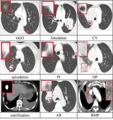
imaging signs of lung diseases (CISL). We summarized nine categories of CISLs, which are illustrated in Fig. 1 and explained in the following. Notice that this taxonomy is neither complete nor widely accepted at present, but these CT signs are really often encountered and widely used in the diagnosis of lung diseases.

1. Grand Grass Opacity (GGO): GGO can be characterizedby areas of hazy increased attenuation of the lung with preservation of bronchial and vascular margins [1]. It isassociated with the adenocacinoma of lung and bronchioloalveolar carcinoma [2], [3].

Fig 1.1 nine categories of CISL.

2. Lobulation: Lobulation is dependent on the ingrowth ofconnective tissue septet containing fibroblasts derived from perithymic mesenchyme [4], which indicates a malignant lesion [5].

3. Cavity and Vacuolous (CV): Both cavity and Vacuolous arehollow spaces within the tissue. We can regard Vacuolous as little cavity. Vacuolous is associated with the adenocacinoma and bronchioloalveolar carcinoma, while cavity is associated with the tumors larger than 3 cm [6], [7].

4. Spiculation: Spiculation is a stellate distortion caused bythe intrusion of cancer into surrounding tissue [8].

5. Pleural Indentation (PI): PI is caused by the contractionof scar affected by the tumor, which is associated with most peripheral adenocacinoma containing a central or subpleural anthracotic and fibrotic focus [9].

6. Obstructive Pneumonia (OP): OP can be characterizedby the following appearances: 1) alveolar septum has not been completely destroyed by tumor, 2) alveolar wall is thin, and 3) alveolus contains gas. This feature is associated with the alveolar carcinoma, lymphoma, pulmonary infarction, and pulmonary edema [10].

7. Calcification: Calcification is the deposition of insolublesalts of calcium and magnesium. Its morphology and distribution are important for discriminating between benign lung diseases and malignant ones. The coarse, dense, and popcorn-like calcification indicates benign lesions, while the calcification located in the center of lesions, spotted, and appearing irregularly suggests malign lesions [11].

(3)

International Journal of Innovative Research in Science,

Engineering and Technology

9. Bronchial Mucus Plugs (BMP): BMP can be representedby focal opacities. Its density varies from liquefied densityto higher than 100 Hounsfield Units (HU). It is associated with the allergic bronchopulmonary aspergillosis [13].

In a previous preliminary work [14], we began to investigate the problem of recognizing the CISLs contained in the ROIs in lung CT images, where four CISL categories including GGO, cavity, speculation, and calcification were considered. In this paper, we expand the number of CISL categories to nine and propose a new feature selection method based on Fisher criterion and genetic optimization for tackling the problem with the help of KPCA. The proposed feature selection method is called FIG for short. It cooperates with each of five commonly used classifiers, including SVM, Bag, NB, k-NN, and Ada, to fulfill the CISL recognition task. We conducted the experiments to demonstrate the effectiveness of the proposed FIG feature selection method as well as CISL recognition approach.

II. EXISTING SYSTEM

We review the previous works on the image classification and the feature selection in the medical image community. For the former problem, we restrict our discussions on lung CT images. For the latter problem, since there is not much related work specific to lung CT images, we expand our view to include other types of medical images.

Fig2.1The flowchart of detection of the location affected area

Fig2.1. a) Original image, (b) histogram equalization from (a), (c) adaptive thresholding operation on (b), and (d) region selection by center C.

The works on lung CT image classification can be divided into three categories according to their purposes: 1) the discrimination between normal and abnormal lung tissues, 2) the identification among visual patterns of specific lung diseases, and 3) the classification of different types of lung lesions. In the first category of works, many methods are presented for nodule detection and GGO detection. They are usually adopted in the final stage of detection systems to decide whether a candidate is true or false. In the second category of works, the explored lung diseases include diffuse parenchyma lung disease (DPLD), chronic obstructive pulmonary disease, and interstitial lung disease (ILD). Although the purposes of three categories of works are different, the frameworks of classification systems are similar in principle, which are usually composed of two components: feature extractor and classifier.

(4)

International Journal of Innovative Research in Science,

Engineering and Technology

second type of features are textural features, such as run-length features [20], [23], local binary patterns (LBP) [21], co occurrence features [23], [24], [27], [32], multiple text on based features [33], vector quantization generating texture descriptor [28], histogram of oriented gradients (HOG) features [21], and wavelets [29]. The third type of features is intensity-based ones. We have gradient magnitude features [16], edge-gradient features [31], CT value histogram (CVH) [21], and intensity distributions [27]. Among the three types of features, the geometric features are mainly used on the lesions having the fixed geometrical properties. The other two types of features, especially textural features, are used more often.

HISTOGRAM EQUALISATION: This method usually increases the global contrast of many images, especially when the usable data of the image is represented by close contrast values. Through this adjustment, the intensities can be better distributed on the histogram. This allows for areas of lower local contrast to gain a higher contrast. Histogram equalization accomplishes this by effectively spreading out the most frequent intensity values.

The method is useful in images with backgrounds and foregrounds that are both bright or both dark. In particular, the method can lead to better views of bone structure in x-ray images, and to better detail in photographs that are over or under-exposed. A key advantage of the method is that it is a fairly straightforward technique and an invertibleoperator. So in theory, if the histogram equalization function is known, then the original histogram can be recovered. The calculation is not computationally intensive. A disadvantage of the method is that it is indiscriminate. It may increase the contrast of background noise, while decreasing the usable signal. The 8 bit gray scale of histogram is shown in below table.

Table1.1. 8 bit histogram table The general histogram equalization formula is:

ADAPTIVE THRESHOLDING: Thresholding is used to segment an image by setting all pixels whose intensity values are above a threshold to a foreground value and all the remaining pixels to a background value.

Whereas the conventional thresholding operator uses a global threshold for all pixels, adaptive thresholding changes the threshold dynamically over the image. This more sophisticated version of thresholding can accommodate changing lighting conditions in the image, e.g. those occurring as a result of a strong illumination gradient or shadows.

There are two main approaches to finding the threshold: (i) the Chow and Kaneko approach and (ii) local thresholding. The assumption behind both methods is that smaller image regions are more likely to have approximately uniform illumination, thus being more suitable for thresholding. Chow and Kaneko divide an image into an array of overlapping sub images and then find the optimum threshold for each sub image by investigating its histogram. The threshold for each single pixel is found by interpolating the results of the sub images.

An alternative approach to finding the local threshold is to statistically examine the intensity values of the local neighborhood of each pixel. The statistic which is most appropriate depends largely on the input image. Simple and fast functions include the mean of the local intensity distribution,

the median value,

(5)

International Journal of Innovative Research in Science,

Engineering and Technology

The size of the neighborhood has to be large enough to cover sufficient foreground and background pixels, otherwise a poor threshold is chosen. On the other hand, choosing regions which are too large can violate the assumption of approximately uniform illumination. This method is less computationally intensive than the Chow and Kaneko approach and produces good results for some applications.

III. PROPOSED SYSTEM

Medical imaging is one of the most important tools in modern medicine; different types of imaging technologies such as X-ray imaging, ultrasonography, biopsy imaging, computed tomography, and optical coherence tomography have been widely used in clinical diagnosis for various kinds of diseases. However, in clinical applications, it is usually time-consuming to examine an image manually. Moreover, as there is always a subjective element related to the pathological examination of an image by human physician, an automated technique will provide valuable assistance for physicians. A large focus with respect to medical image analysis has been on automated image classification. Many recent studies have revealed that medical images can be properly classified if suit-able image feature descriptions are chosen [1-3]. These researches demonstrated that by combining different imagedescription features, it is possible to improve medical image classification performance.

Although the classifiers which can provide multi-class classification such as support vector machines (SVM) and neural networks are usually selected for medical image classification [4], one-class classifiers (OCC) [5] that can work on the samples seen are, so far, more appropriate for medical image classification task. One-class classification is also often called outlier (or novelty) detection as the learning algorithms are used to differentiate between data that appears normal and abnormal with respect to the distribution of the training data. This principle of one-class classification is thus appropriate with respect to medical diagnosis and in disease versus no-disease problems.

FEATURE SELECTION METHOD BASED ON FISHERCRITERION AND GENETIC OPTIMIZATION In essence, the feature selection problem is to find out the best feature subset in the power set of features. Therefore, it involves two subproblems: 1) how to evaluate feature subset and 2) how to implement search. For the search algorithm, the GA is a popular and good choice. But most of GA-based feature selection algorithms measure the quality of feature subset by its classification accuracy rate (CAR). In the following descriptions, a feature subset is called an individual, and the quality of it is called its fitness, according to GA’s terminology. Using the CAR as the individual fitness has two disadvantages. First, it makes the feature selection method depend on the underlying classifier. The optimal feature subset generated for one classifier may not be necessarily appropriate to another one. Second, for getting the individual fitness, the classifier must be retrained with the corresponding feature subset and then used to perform classification on the dataset to obtain the CAR. This procedure of fitness evaluation is obviously time consuming and leads to the unsatisfactory efficiency of GA search. In order to solve the two shortcomings above, our FIG method introduces the Fisher discriminative criterion [49] to measure the individual fitness in the GA-based optimum search. Although both the Fisher criterion and the GA algorithm have been explored in previous works on feature selection, respectively, this strategy of ours for combining them is the first one to our knowledge.

Furthermore, in most of GA-based feature selection methods, the feature selection result is represented by a binary string. Each bit in the string corresponds to a feature, where the value 1 indicates that the feature is selected and 0 indicates that the feature is discarded. Different from these methods, we assign a weight in [0, 1] to each feature and evolve the weights. It is more reasonable and more accurate for measuring the importance degree of a feature than the hard value of 0 or 1. After the weight evolution is completed, the feature whose weight exceeds a threshold is chosen as a member of the optimal feature subset.

1. Fitness Function Based on Fisher Criterion:

(6)

International Journal of Innovative Research in Science,

Engineering and Technology

2. Genetic Optimization for Feature Selection:

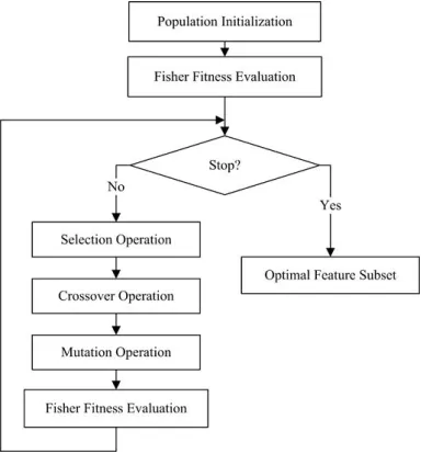
Under GA optimization framework, the main components of our FIG algorithm include population initialization, fitness evaluation, selection, crossover, mutation, and termination judgment. The corresponding flowchart of the algorithm is illustrated in Fig. 2, where “Fisher Fitness Evaluation” means “the fitness evaluation based on Fisher criterion.” The fitness evaluation method has been presented in the last section. The details of other components are given as follows.

Population Initialization: In the GA algorithms, all theindividuals in each generation construct the population. Each individual is encoded as a binary string, which is thought to be the individual’s chromosome. As described previously, an individual in the FIG algorithm is a feature-weight vector. Suppose the weights are required to be accurate to p

decimal places, then the closed interval [0, 1] needs to be divided into 10p equal parts.

Selection Operator: The selection operator is used to select the parent individuals which will participate in producing offsprings for the next generation. Here, the commonly used roulette wheel selection technique [50] is used.

Fig 3.1Flowchart for fisher criterion

Crossover Operator: The crossover operator is used tocreate new individuals by recombining the genes of the chromosomes of the selected two parents. Considering that there are different types of features for selection and at least one feature of each type should be selected, the multipoint crossover is per-formed. Actually, we divide the chromosome of an individual into several parts, each of which is corresponding with a type of features. Then, we perform the single-point crossover in each part of the chromosome, respectively.

The probability of crossover affects the search ability and the convergence speed of GA. In this study, we follow to adopt the adaptive probability of crossover.

Mutation Operator: The mutation occurs right after thecrossover is completed. It is performed by inversing one bit in each part of an individual’s chromosome to create a child. Similar to the processing in the crossover, each part of the chromo-some is corresponding with a type of features, and the mutation probability is also adjusted adaptively.

Termination Judgment: The algorithm will be terminatedwhen it converges or the predefined maximum number of generations is reached. The condition that we use to judge whether the algorithm converge is: The difference between the maximum fitness values of adjacent two generations does not exceed an infinitesimal (denoted as ε) after m

(7)

International Journal of Innovative Research in Science,

Engineering and Technology

FEATURE EXTRACTION

We consider four types of ROI features, including the bag-of-visual-words based on the HOG (B-HOG), the wavelet features, the LBP, and the CVH. We have 18-D B-HOG features, 26-D wavelet features, 96-D LBP features, and 40-D CVH features. Total 180 features are extracted. The details of each type of features are given as follows.

1)B-HOG: The HOG feature is a texture descriptor describing the distribution of image gradients in different orientations. Following the HOG feature extraction scheme of Dalal and Triggs [52], we divide a ROI into smaller rectangular blocks of 8 × 8 pixels and further divide each block into four cells of 4 × 4 pixels. An orientation histogram which contains nine bins covering a gradient orientation range of 0–180° is computed for each cell. Then, a block is represented by the linking of the orientation histograms of cells in it. This means a 36-D HOG feature vector is extracted for each block.

The commonly used image representation based on HOG features is to join the feature vectors of all the blocks in the image in sequence. This kind of HOG-based image representation strategy requires that all the images have the same size, or else the dimensions of resultant feature vectors will be diverse for different images. But the size of ROIs in lung CT images varies with different patients and different pathological lesions. So this widely used strategy is not applicable in this study. To solve this problem, we adopt the bag-of-visual-words [53] on HOG features as the ROI representation. However, different from the original bag-of-visual-words method, we use a clustering algorithm based on Gaussian mixture modeling (GMM) [54], instead of the k-means algorithm, to generate more ac-curate visual words. In this paper, total 18 visual words are obtained.

The 36-D HOG feature vector of each block is mapped to the visual word corresponding to the highest likelihood for it. Then, the number of HOG feature vectors assigned to each visual word is accumulated and normalized by the number of all the HOG feature vectors to form a 18-D histogram representation of the ROI.

2)Wavelet Features: Wavelets are important and commonlyused feature descriptors for texture analysis, due to their effectiveness in capturing localized spatial and frequency information and multi resolution characteristics [55]. In this paper, the ROIs are decomposed to four levels by using 2-D symlets wavelet be-cause the symlets wavelet has better symmetry than Daubechies wavelet and more suitable for image processing [56]. Then, the horizontal, vertical, and diagonal detail coefficients are extracted from the wavelet decomposition structure. Finally, we get the wavelet features by calculating the mean and variance of these wavelet coefficients.

3)LBP: The LBP feature is a compact texture descriptor inwhich each comparison result between a center pixel and one of its surrounding neighbors is encoded as a bit [57]. In this way, we can get an integer for each pixel. Then, the frequency of each integer is figured out on the ROI level to obtain the corresponding feature vector.

The neighborhood in the LBP operator can be defined very flexibly by using circular neighborhoods and the bilateral interpolation of pixel values. These kinds of neighborhoods can be denoted by (P, R), which means we evenly sample P

neighbors on the circle of radius R around the center pixel. The corresponding LBP features will be denoted as LBP(P,

R) in the following descriptions. We consider multiple P and R to get multi scale LBP features.

4) CVH Features: CVH means the histogram of CT values. Inlung CT images, the CT values of pixels are expressed in HU. We compute the histogram of CT values over each ROI. The number of bins in the histogram is determined by experiments. In fact, we obtain various CVHs with different numbers of bins. Each CVH is tested for classification under k-NN classifier, and the corresponding CAR is calculated. Then, the number of bins, which brings the highest CAR, is adopted. This choice will keep unchanged for all the experiments.

ROI CLASSIFICATION

Five classifiers, including SVM, Bag, NB, k-NN, and Ada, are, respectively, tested for cooperating with the selected features to classify ROIs into CISL categories. These classifiers are implemented by using the corresponding functions in WEKA [58], a machine-learning library in java. The name of these functions are: 1) “SMO” (SVM), 2) “Bag,” 3) “NB,” 4) “IBk” (k-NN, k = 1and Euclidean distance are adopted), 5) “AdaBoostM1”(Ada, using REPTree as weak learner).

(8)

International Journal of Innovative Research in Science,

Engineering and Technology

IV. EXPERIMENTS

Ensemble of one-class classifiers

Ensemble learning is concerned with mechanisms to combine the results of a number of weak learning systems to produce better learning performance. Several methodologies exist for creating an ensemble classifier from individual classifiers; a survey on the design of multiple classifier systems can be found in [6]. It has been demonstrated that combining classifiers can also be effective for one-class classifiers. The existing classifier combination strategies can also be used in one-class classifiers. Because for one - class classifiers, information concerning only one class is available; thus, the combining of one-class classifiers is more difficult. Tax and Duin investigated the influence of feature sets and the types of one-class classifiers for the best choice of the combination rule [30]. A bagging-based one-class support vector machine ensemble method was proposed in [31]. A dynamic ensemble strategy based on structural risk minimization [32] was proposed by Goh et al. for multi-class image annotation [7]. Recently, some research results have revealed that creating a one-class classifier ensemble from different feature subsets can provide better performance. Predict et al. [33] also used an ensemble of one-class SVMs to create a ‘high-speed payload-based’ anomaly detection system, in which the features were first extracted and clustered and the OCSVM ensemble was then constructed based on the clustered feature subsets. A biometric classification sys-tem combining different biometric features was proposed by Bergamini et al. [8], where the one-class SVMs in the ensemble were trained by the data from different people. The feature subset strategy provides diversity with respect to the base classifiers, and some researchers emphasize the importance of measuring diversity in ensembles so as to improve classification performance [9,34].

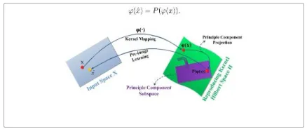
KPCA and pattern reconstruction via pre-image

The traditional (linear) PCA tries to preserve the greatest variations of data by approximating data in a principle component subspace spanned by the leading eigenvectors, noises or less important data variations will be removed. Kernel PCA inherits this scheme; however, it performs linear PCA in the kernel feature space Hκ . Suppose X

⊂Rn is the original input data space and Hκ is a reproducing kernel Hilbert space (RKHS) (also called feature space)

associated to a kernel function κ (x, y) =< ϕ(x), ϕ(y) >, where x, y∈ X. ϕ(·) is a mapping induced by κ that ϕ(x) : X →

Hκ . Given a set of patterns {x1, x2, . . . ,xN } ∈ X, kernel PCA performs the traditional linear PCA in Hκ . Similar to the linear PCA, KPCA also has the eigendecom-position.

Figure 4.1 Illustration of KPCA pre image learning. The samplexin the original space is first mapped into the kernel

space by kernel mappingϕ(·),then PCA is used to project ϕ(x) into P(ϕ(x)), which is a point in a PCA subspace. Pre image learning is used to find the pre image xˆ of x in the original input space from P(ϕ(x)).

A. Experimental Setup

1) Dataset: The instances of nine categories of CISLs werecollected from the Cancer Institute and Hospital at the Chinese Academy of Medical Sciences. The lung CT images were acquired by CT scanners of GE Light Speed VCT 64 and Toshiba Aquilion 64 and saved in DICOM 3.0 format. The slice thickness is 5 mm, the image resolution is 512 ×

512, and the in-plane pixel spacing ranges from 0.418 to 1 mm (mean: 0.664 mm).

(9)

International Journal of Innovative Research in Science,

Engineering and Technology

classification performance is avoided. Table I lists the numbers of ROI examples in five data subsets and the numbers of patients for each CISL category, where S1–S5 denote the first to the fifth subsets, respectively, and NoP means “the number of patients.”

2)Evaluation Criterion: The performance of CISL recognition is evaluated by the SE and SP, CAR, and confusion matrix (CM).The SE and SP are widely used in the medical image classification community. They are essentially two measurements of performance of binary classifiers paper; we use them to reflect the ability of our CISL recognizer for discriminating one CISL category from any other categories. If a positive example for a CISL category can be recognized correctly by the algorithm, we call it “true positive”; otherwise, we call it “false negative”. The meanings of “true negative” and “false positive” are defined similarly. Let TP, TN, FP, FN be the number of true positives, true negatives, false positives, and false negatives for a CISL category, respectively. Then, the SE and SP of the classifier for this category are measured as

TP/(TP+FN) and TN /(TN+FP), respectively.

Our CISL recognition problem is actually a multiclass classification problem. So we use the CAR to give an overall measurement of performance of our CISL recognizer. It is the ratio of the number of correctly classified examples to the number of all examples.

The CM is used to summarize the tendency for our CISL recognizer to classify a pattern into a correct class or any of other wrong classes.

3) Parameter Setting: Two groups of parameters of our approach were set up through experiments. The first group of parameters is those in the proposed FIG feature selection method.

B. Experimental Results

1) Results of Feature Selection and CISL Recognition: Weconducted feature selection and ROI classification experiments. Table IV shows the numbers of features selected from original 180 features and the determined weight threshold for selecting features in each round of fivefold cross-validation experiments.

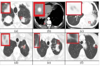
Fig 4.2 Examples of classified CISLs: (a) lobulation noised by blood vessel; (b) calcification identified difficultly; (c) and (d) easy confused AB and CV; (e) and (f) easy confused spiculation and PI.

We carefully analyzed the reasons behind wrong classification results from the recognizer established by combining selected features and the SVM. The reasons are illustrated in Fig. 3 and explained as follows, where the lesions are indicated by the smaller rectangles in lung CT images and magnified to display clearer in the bigger rectangles overlapping on the images. 1) Some CISLs are noised by blood vessels surrounding them, as shown in Fig. 3(a). 2) Some CISLs are so small and hazy that it is difficult to recognize them even by radiologists, as shown in Fig.4.

2)Comparisons With Independent Feature Space and Original Full Set of Original Features: In order to prove the necessityof feature selection, we further conducted the CISL recognition by using each type of original features and the full set of original features, respectively.

(10)

International Journal of Innovative Research in Science,

Engineering and Technology

the ARG. We recorded the CISL recognition performance and computation time of FIG and ARG algorithm, respectively. All the experiments were performed on a computer with 2.33-GHz CPU and 4-GB Memory.

Fig.4.3. Comparisons of CARs for each considered classifier between ARG and FIG feature selection methods.

We further conducted the paired t-test analysis [59] to deter-mine whether there is a significant difference in effectiveness between FIG and ARG. The resultant two-tailed p values for SVM, Bag, NB, k-NN, and Ada are 0.823, 0.334, 0.319, 0.957, and 0.858, respectively. Usually p <0.05 is accepted as significant. So we conclude that although the FIG behaved a little better than the ARG on the average, the difference in the effectiveness between them is not significant.

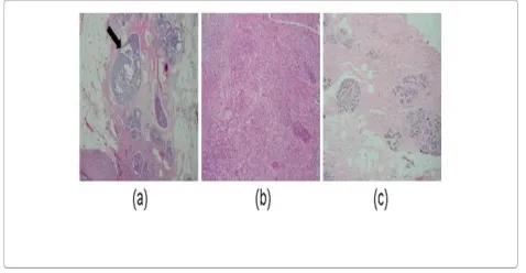
Figure 4.4 Typical image instances. (a) Carcinomain situ: tumor confined to a well-defined small region, usually a

duct (arrow). (b) Invasive: breasttissue completely replaced by the tumor. (c) Normal: normal breast tissue, with ducts and finer structures.

V. CONCLUSION

In this paper, a classification scheme based on a one-class KPCA model ensemble has been proposed for the classification of medical images. The ensemble consists of one-class KPCA models trained using different image features from each image class, and a proposed product combining rule was used for combining the kernel PCA models to produce classification confidence scores for assigning an image to each class. The effectiveness of the proposed classification scheme was verified using a breast cancer biopsy image dataset and a 3D OCT retinal image set. The proposed classification scheme obtained high classification accuracy on the tested image sets.

(11)

International Journal of Innovative Research in Science,

Engineering and Technology

optimization methods or adaptive algorithms should be considered for searching the optimal parameters of KPCA models.

A feature selection method is presented based on Fisher criterion and genetic optimization, which is called FIG for short. The Fisher criterion is applied to evaluate feature selection results, based on which a genetic optimization algorithm is developed to find out the optimal feature subset from candidate features. As demonstrated by the experimental results, our FIG method can bring more effective recognition results at the satisfactory computation costs, compared with single type of features and the full set of original features. Furthermore, it brought slightly better recognition performance and much better computation efficiency than the commonly used genetic feature selection method based on classification accuracy rate. Another advantage of the FIG is that it is independent of the classifiers; it is required to be performed only once to select the features suitable for all the considered classifiers.

In the future, we want to add some image preprocessing steps to further improve the performance of our CISL recognizer. We can filter the blood vessels to get rid of the confusion between vessels and CISLs. We can also enhance the regions wrapping CISLs to make the visual appearance of CISLs clearer and thus increase the possibility of correct classification.

REFERENCES

[1] G. Battista, C. Sassi, M. Zompatori, D. Palmarini, and R. Canini, “Ground-glass opacity: Interpretation of high resolution CT findings,” La

Radiolo-giaMedica, vol. 106, pp. 425–442, 2003.

[2] Z. G. Yang, S. Song, and S. Talcashima, “High-resolution CT analysis of small lung adenocarcinoma revealed on screening helical CT,” Amer.

J.Roentgenol., vol. 176, no. 6, pp. 1399–1407, 2001.

[3] T. Aoki, Y. Tomoda, H. Watanabe, H. Nakata, T. Kasai, H. Hashimoto, M. Kodate, T. Osaki, and K. Yasumoto, “Peripheral lung adenocarcinoma: Correlation of thin-section findings with histologic factors and survival,” Radiology, vol. 220, pp. 803–809, 2001.

[4] J. J. T. Owen, D. E. McLoughlin, R. K. Suniara, and E. J. Jenkinson, “The role of mesenchyme in thymus development,” Current Topics

Microbiol.Immunol., vol. 251, pp. 133–137, 2000.

[5] M. R. Melamed, B. J. Flehinger, M. B. Zaman, R. T. Heelan, W. A. Perchick, and N. Martini, “Screening for lung cancer: Results of the memo-rialsloan-kttering study in New York”, Chest, vol. 86, no. 1, pp. 44–53, 1984.

[6] C. V. Zwirewich, S. Vedal, R. R. Miller, and N. L. Muller,¨ “Solitary pulmonary nodule: High-resolution CT and radiologic-pathologic corre-lation,” Radiology, vol. 179, no. 2, pp, 469–476, 1991.

[7] S. F. Huang, R. F. Chang, D. R. Chen, and W. K. Moon, “Characterization of spiculation on ultrasound lesions,” IEEE Trans. Med. Imag., vol. 23, no. 1, pp. 111–121, Jan. 2004.

[8] M. Noguchi and Y. Shimosato, “The development and progression of adenocarcinoma of the lung,” Cancer Treatment Res., vol. 72, pp. 131– 142, 1995.

[9] T. V. Colby and C. Lombard. “Histiocytosis X in the lung,” Human Pathol., vol. 14, no. 10, pp. 847–856, 1983.

[10] V. J. Lowe, J. W. Fletcher, L. Gobar, M. Lawson, P. Kirchner, P. Valk, J. Karis, K. Hubner, D. Delbeke, E. V. Heiberg, E. F. Patz, and R. E. Coleman, “Prospective investigation of positron emission tomography in lung nodules,” J. Clin. Oncol., vol. 16, no. 3, pp. 1075–1084, 1998. [11] K. S. Lee, Y. Kim, and S. L. Primack, “Imaging of pulmonary lymphomas,” Amer. J. Roentgenol., vol. 168, no. 2, pp. 339–345, 1997.

[12] J. W. Gurney, “Determining the likelihood of malignancy in solitary pulmonary nodules with Bayesian analysis: Part 1. Theory,” Radiology, vol. 186, no. 2, pp. 405–413, 1993.

[13] J. J. Erasmus, H. I. McAdama, and J. H. Connolly, “Solitary pulmonary nodules: Part II. Evaluation of the indeterminate nodule,”

Radiographics, vol. 20, no. 1, pp. 59–66, 2000.

[14] L. Song, X. Liu, L. Ma, C. Zhou, X. Zhao, and Y. Zhao, “Using HOG-LBP features and MMP learning to recognize imaging signs of lesions,” in

Proc. Comput.-Based Med. Syst., 2012, pp. 1–4.

[15] X. Ye, X. Lin, G. Beddoe, and J. Dehmeshki. “Efficient computer-aided detection of ground-glass opacity nodules in thoracic CT images,” in

Proc.29th Annu. Int. Conf. IEEE Eng. Med. Biol. Soc., 2007, pp. 4449–4452.

[16] T. W. Way, B. Sahiner, H. P. Chan, L. Hadjiiski, P. N. Cascade, A. Chughtai, N. Bogot, and E. Kazerooni, “Computer-aided diagnosis of pul-monary nodules on CT scans: Improvement of classification performance with nodule surface features,” Med. Phys., vol. 36, no. 7, pp. 3086– 3098, 2009.

[17] H. Chen, Y. Xu, Y. Ma, and B. Ma, “Neural network ensemble-based computer-aided diagnosis for differentiation of lung nodules on CT im-ages clinical evaluation,” Acad. Radiol., vol. 17, no. 5, pp. 595–602, 2010.

[18] H. U. Kauczor, K. Heitmann, C. P. Heussel, D. Marwede, T. Uthmann, and M. Thelen, “Automatic detection and quantification of ground-glass opacities on high-resolution CT using multiple neural networks: Com-parison with a density mask,” Amer. J. Roentgenol., vol. 175, no. 5, pp. 1329–1334, Nov. 2000.

[19] K. G. Kim, J. M. Goo, J. H. Kim, H. J. Lee, B. G. Min, K. T. Bae, and J. G. Im, “Computer-aided diagnosis of localized ground-glass opacity in the lung at CT: initial experience,” Radiology, vol. 237, no. 2, pp. 657–661, 2005.