Geometric Number of Planar Graphs

Geometric Number of Planar Graphs

H. R. Bhapkar 1, Dr. J. N. Salunke2, A. H. Bhapkar3

Associate Professor, Department of Mathematics, Smt. Kashibai Navale College of Engg., Pune, Maharashtra, India1

Professor, Department of Mathematics, S. R. T. M. U. Nanded, Maharashtra, India2

Assistant Professor, Department of Physics, Sinhgad College of Engineering, Pune, Maharashtra, India3

ABSTRACT: With the help of the geometric dual of graphs, this paper defines SD graphs and proves the related results. This paper proves “How many minimum or maximum numbers of edges are there for an SD graph with n vertices?” Therefore, the first geometric number and the greatest geometric number come into the centre of attention. It proves formulae for geometric numbers as well as the number of graphs with the particular number of vertices.

KEYWORDS:SD Graphs, First geometric number, Greatest geometric number.

I. INTRODUCTION

In this section, we present a brief survey of those results of graph theory, which we shall need later. The reader is referred to [5, 6, 9, 10, 11] for a fuller treatment of the subject.

A. GRAPHS

A graph G is an ordered pair (V (G), E (G) ) where i) V(G) is a non empty finite set of elements , known as vertices. V (G) is known as vertex set. ii) E(G) is a family of unordered pairs ( not necessarily distinct ) of elements of V, known as edges of G. E(G) is known as Edge set.

Each vertex of graph G is represented by a point or small circle in the plane. Every edge is represented by a continuous arc or straight line segment. A certain pairs of vertices of graph are joined by two or more edges, such edges are known as multiple or parallel edges. An edge joining a vertex to itself, is called a loop. A graph without loops or multiple edges is called a simple graph. Non-simple graphs are known as multiple graphs. The degree or valency of a vertex v of graph G is the number of edges incident at that v. It is denoted by d (v). A vertex of degree 1 is called a pendent vertex. A vertex of zero degree is said to be isolated vertex. An edge, whose one end vertex is a pendant vertex, is known as pendant edge [9].

B. PLANAR GRAPH

A graph G is a planar graph if it is possible to represent it in the plane such that no two edges of the graph intersect except possibly at a vertex to which they are both incident. Any such drawing of planar graph G in a plane is a planar embedding of G [4].

If x any point in the plane of a planar graph that is neither a vertex nor a point on an edge, the set of all points in the plane that can be reached from x by traversing along a curve that does not have a vertex of the graph or a point of an edge as an intermediate point, is the region of the graph that contains x. Thus the plane graph G partitions the plane into the different regions of G. Among these regions there is exactly one region whose area is not finite, is called exterior or infinite region. Every other region is an interior region. The boundary of a region is a sub-graph formed by the vertices and edges encompassing that region. If the boundary of the exterior region of a planar graph is a cycle, that cycle is known as the maximal cycle of that graph. The degree of the region is the number of edges in a closed walk that encloses it. The region formed by three edges is known as triangular region. The region formed by four edges is known as rectangular region [6].

C. GEOMETRIC DUAL

Let G be a plane graph with n regions or faces say R1, R2, R3, . . .Rn . Let us place points (say vertices) V1, V2, V3, . . .

Vn , one in each of the regions. Let us join these vertices Vi according to the following procedure.

i) If two regions Ri and Rj are adjacent then draw a line joining vertices Vi and Vj that intersect the common edge

between Ri and Rj exactly once.

ii) If there are two or more edges common between Ri and Rj , then draw one line between vertices Vi and Vj for each

of the common edges.

iii) For an edge ‘e’ lying entirely in one region say Ri, draw a self loop at pendant vertex Vi intersecting e exactly once.

By this procedure, we obtain a new graph G* consisting of V1, V2, V3, . . . Vn vertices and edges joining these

vertices. Such a graph G* is called a geometric dual of G (a dual of G) [2]. Theorem 1.2: The geometric dual of a planar graph is planar [9].

1.4 * isomorphism of Graphs

Two graphs are said to be *isomorphic if their geometric duals are isomorphic. Every graph is * isomorphic to itself. The definition is symmetric, and if G1 and G2 are *isomorphic to G2 and G3, respectively, then G1 and G3 are *

isomorphic. Thus *isomorphism is an equivalence relation [1].

Suppose two graphs are * isomorphic, then it is clear that the two graphs must have same number of edges and same number of regions formed by an equal number of edges. There is no any condition on number of vertices of the two graphs. Thus these conditions are necessary for two graphs to be *isomorphic. However, these conditions are not sufficient [3].

II. RELATED WORK

A. SD GRAPHS

A planar graph G is said to be SD graph if it’s geometric dual G* is a simple graph. The geometric dual of the null graph is a null graph, so every null graph is a SD graph. The complete graph on 4 vertices is SD graph. Graphs K2 and

K3 are not SD graphs.

Theorem 2.1 A planar graph G is a SD graph if and only if any two distinct regions of G do not have two or more

boundary edges common and no bridges.

Proof: Suppose planar graph G is a SD graph. So Graph G* is a simple graph. G* is free from loops and parallel edges. By the definition of geometric dual, G has no bridges. Two parallel edges are present in the dual graph if the graph has two boundary edges common between their regions. As G* has no parallel edges, so two distinct regions of G do not have two or more boundary edges common.

Conversely, suppose G has no bridges. So G* has no loops. Moreover, two distinct regions of G do not have two or more boundary edges common, so G* has no parallel edges. Therefore, G* has no loops and parallel edges. Thus, graph G* is a simple graph. Hence, graph G is SD graph. □

Theorem 2.2 Every wheel graph on n ≥ 4 vertices is SD graph.

Proof: Every wheel graph is a simple graph and its geometric dual is also a wheel graph. Therefore, every wheel graph is a SD graph. □

B. THE GEOMETRIC NUMBER OF GRAPHS

Let Gn be a simple planar connected graph with n vertices. The non-zero integer m is called the geometric number of

graph Gn if there exist at least one graph with m number of edges, whose geometric dual is a simple graph. The first and

i. First Geometric Number of Graphs

Let Gn be a simple planar connected graph with n vertices. The smallest non-zero integer m is called the first geometric

number of graph Gn if there is at least one graph with m number of edges whose geometric dual is a simple graph. It is

denoted by F (Gn). The first geometric number of graph G4 is 6.

ii. Greatest Geometric Number of Graphs

Let Gn be a simple planar connected graph with n vertices. The greatest non-zero integer m is called the greatest

geometric number of graph Gn if there is at least one graph with m number of edges whose geometric dual is a simple

graph. It is denoted by G (Gn). The greatest geometric number of graph K4 is 6.

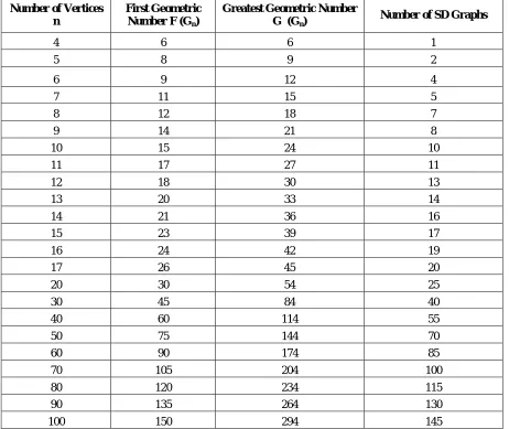
Let Gn be a SD graph with n vertices. Consider the following table which represents

n = number of vertices of graph, F (Gn) = First geometric number of graph with n vertices,

G (Gn) = Greatest geometric number of graph with n vertices.

Number of Vertices n

First Geometric Number F (Gn)

Greatest Geometric Number G (Gn)

Number of SD Graphs

4 6 6 1

5 8 9 2

6 9 12 4

7 11 15 5

8 12 18 7

9 14 21 8

10 15 24 10

11 17 27 11

12 18 30 13

13 20 33 14

14 21 36 16

15 23 39 17

16 24 42 19

17 26 45 20

20 30 54 25

30 45 84 40

40 60 114 55

50 75 144 70

60 90 174 85

70 105 204 100

80 120 234 115

90 135 264 130

100 150 294 145

The complete graph on 4 vertices is the only graph in which the first and the greatest geometric numbers are equal. There are unique graphs with geometric numbers 6, 8 and 10. There is no any graph whose geometric number is 7. There exist graphs whose greatest geometric number is 3p or the first geometric number is 3p. If H is a graph with n vertices whose first geometric number is 3p then there is no any graph on n vertices whose first geometric number is 3p – 1. But there exists a graph on n + 1 vertices whose first geometric number is of the form 3p – 1 and there is no any graph whose greatest geometric number is 3p – 1.

Theorem 2.3 If Gn is a simple planar connected graph on n ≥ 4 vertices, then the first geometric number of Gn is















2

n

n

Proof: If n = 4, then F (G4) = 6 and





2 4 4

2      

     n n

Therefore the result is true for

n = 4.

Assume that result is true for n = k, where k = 4, 5,…, n -1. Case 1:n is an odd integer.

n - 1 is even. Add one vertex say x in the inner circle of Gn-1 between vertices a and b, join x to vertices u or v as

shown in figure 2.3 (A). The new graph is denoted by Gn.

A B

Fig. 1 An illustration of the First Geometric Number of Graphs

In figure A, there are an odd number of vertices. Inner and outer circles of graph have        2 1

n _{+1 and}        2 1 n _vertices

respectively. There is an even number of vertices in figure B. Inner and outer circles of graph have        2 1 n _vertices.

















Case 2:n is an even integer.

n – 1 is an odd integer. The inner circle of Gn-1 has one less vertex then that of the outer circle. Add one vertex say x

















Hence the proof. □

Theorem 2.4 If Gn is a simple planar connected graph on n ≥ 4 vertices, then the greatest geometric number of Gn is

3n – 6.

Proof: Let Gn be a simple planar connected graph onn ≥ 4 vertices. By the definition of the greatest geometric number

of a graph, Gn must have triangular regions. Therefore, Gn is the maximal planar graph. We know that the geometric

dual of the maximal planar graph is a simple graph and it has 3n – 6 edges. Thus, the greatest geometric number of graph Gn is 3n – 6. □

Theorem 2.5 If G is a simple planar connected graph with n ≥ 4 vertices then prove that F (Gn) ≤ G (Gn) and

F (Gn) = G (Gn) only if Gn = K4. Proof: We have









2  

    

 n n and G G n

G

F n n

Assume that result is true for a graph with n-1 vertices. Therefore

6 3 2 1 2 2 6 3 3 9 3 3 2 1 1 9 3 6 ) 1 ( 3 2 1 1                                                 n n n n n n n n n n n n n

Thus F (Gn) < G (Gn) , for all n.

Suppose F (Gn) = G (Gn)

If n is an even integer, then

If n is an odd integer, then 3 13 13 3 12 1 4 6 2 1 2 6 2 1 3 6 3 2 1                      n n n n n n n n n n n n

n = 13/3 is not possible.

Thus F (Gn) = G (Gn) if and only if n = 4. □

Theorem 2.6 The number of graphs with distinct geometric numbers on n ≥ 4 vertices is

        2 5

2n n

.

Proof: We have









2  

    

 n n and G G n

G

F n n

Let p be the number of graphs with distinct geometric numbers on n vertices. Therefore

                 2 5 -2n p } 1 2 {n -6) -(3n p n n III. CONCLUSION

We have defined SD graphs by using the geometric dual of planar graphs and proved few related results. This paper has defined the first geometric number, the greatest geometric number of graphs and proved formulae for it. We have also proved that the number of graphs with distinct geometric numbers on particular number of vertices.

REFERENCES

[1] H. R. Bhapkar and J. N. Salunke, “*isomorphism of Graphs”, International Journal of Mathematical Sciences and Engineering Applications, Vol. 8, No. II, 0973-9424, March 2014.

[2] H. R. Bhapkar and J. N. Salunke, “The Geometric Dual of HB Graph, *outerplanar Graph and Related Aspects”, Bulletin of Mathematical Sciences and Applications, ISSN 2278-9634, Volume 3, No. 3, pp 114-119, August 2014.

[3] H. R. Bhapkar and J. N. Salunke, “Partitions, Haary Graphs and * isomorphism”, International Journal of Pure and Engineering Mathematics, ISSN 2348-3881, Volume 2, No. 2, August 2014.

[4] H. R. Bhapkar and J. N. Salunke, “Proof of Four Color Theorem by Using PRN of Graph” journal of Bulletin of Society for Mathematical Services and Standards ISSN 2277- 8020, Volume 3, No. 2, pp 35-42, Sept. 2014.

[5] Harary, F. “Graph Theory”, Reading, MA: Addison-Wesley, pp. 113-115, 1994.

[6] H. Whitney, “On the Abstract Properties of Linear Dependence”, American Journal of Mathematics, 57 (1935) 509-533. [7] J. A. Bondy and U. S. R. Murty, “Graph Theory with Applications”. Elsevier, Macc Millan, New York - London, 1976. [8] M. O. Albertson and J. P. Hutchinson. “Discrete Mathematics with Algorithms”. Wiley, New York, 1988.

[9] Narsingh Deo, “Graph Theory with Applications To Engineering and Computer Science”, Prentice –Hall of India, 2003. [10] Robin J. Wilson, “Introduction to Graph Theory”, Pearson, 978-81-317-0698-5, 2011.

BIOGRAPHY

Dr. H. R. Bhapkar, M. Sc., SET, Ph. D., Associate Professor, Department of Mathematics, Smt. Kashibai Navale College of Engineering, Pune, Maharashtra, India. He has 17 years teaching experience and published 11 research papers in national and international reputed journals. He has authored 72 books of Engineering Mathematics to different university of India.