Performance Characterization of IP Network-based Control Methodologies for DC Motor Applications.

(1)

ABSTRACT

RICHARDS, TYLER V. Performance Characterization of IP Network-based Control

Methodologies for DC Motor Applications. (Under the direction of Dr. Mo-Yuen Chow.)

Using a communication network, such as an IP network, in the control loop is

increasingly becoming the norm. This process of network-based control (NBC) has potential

profound impact in areas such as: teleoperation, healthcare, military applications, and

manufacturing. However, limitations arise as the communication network introduces delay

that often degrades or destabilizes the control system. Four methods have been investigated

that alleviate the IP network delays to provide stable real-time control. A performance

measure is defined for a case study on a DC motor with a networked proportional-integral (PI)

speed controller with various network delays and noise levels. Matlab simulation results

show that NBC combined with these techniques can successfully maintain system stability,

(2)

(3)

BIOGRAPHY

(4)

ACKNOWLEDGMENTS

(5)

LIST OF FIGURES

Figure 1. Structure of a network-based control system. 2

Figure 2. Structure of GSM. 6

Figure 3. Configuration of networked control system utilizing queuing methodology.

9

Figure 4. Delay compensation algorithm with predictor blocks. 12 Figure 5. Timing diagram for _τsc ₌_τca ₌_δ _. ₁₃ Figure 6. Controller-Plant Modeling with Network Delays. 14 Figure 7. Robust analysis for a general interconnection system. 15 Figure 8. Nominal PI controller step response with ₍ *_, *_{) (25.572,0.995)}

I P

K K = . 19

Figure 9. MSE cost vs. β. 21

Figure 10. P.O. cost vs. β. 21

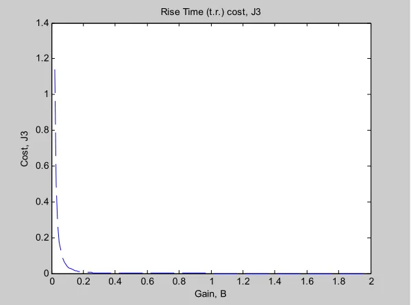
Figure 11. t_r cost vs. β. 22

Figure 12. Histogram for η=0.0001sec RTT delay. 24 Figure 13. Cost vs. β for η=[0.0001,0.001,0.005] network delays. 27 Figure 14. Cost vs. β for η=[0.01,0.05,0.1] network delays. 27 Figure 15. Nominal PI controller vs. GSM step responses for a) η=0.0001 b)

0.001

η = c) η =0.005 d) η=0.01 e) η=0.05 f) η =0.1 seconds.

29

Figure 16. Nominal PI controller vs. Optimal stochastic method step responses for a) η =0.0001 b) η =0.001 c) η =0.005 d) η=0.01 e) η=0.05 f) η=0.1 seconds.

32

Figure 17. Nominal PI controller vs. Queuing methodology step responses for a) 0.0001

η = b) η =0.001 c) η =0.005 d) η=0.01 e) η=0.05 f) 0.1

η = seconds.

35

Figure 18. Nominal PI controller vs. Robust control methodology step responses for a) η =0.0001 b) η =0.001 c) η =0.005 d) η=0.01 e) η=0.05 f) η=0.1 seconds.

(9)

Figure 19. Noise, w k( ) introduced into the control loop. 41

Figure 20. Noise distributions. 41

Figure 21. Typical step response with 5% noise, 0.0001 sec RTT delay. 41

Figure 22. Performance comparison with noise. 42

Figure 23. GSM noise vs. delay performance. 43

Figure 24. Optimal method noise vs. delay performance. 44 Figure 25. Queuing method noise vs. delay performance. 46 Figure 26. Robust methodology noise vs. delay performance. 47

Figure 27. find_beta_sim.mdl 55

Figure 28. lqr_dc_delay_tweak.mdl 64

Figure 29. queue_comp3_sub10.mdl 68

Figure 30. robust_delay1_K3.mdl 72

Figure 31. dkitgui setup screen. 87

(10)

LIST OF TABLES

Table 1. DC motor parameters. 17

Table 2. Optimal β gains for various time delays. 26 Table 3. Performance comparison of four methodologies for different RTT

network delays.

30

Table 4. Queue lengths for various delays. 34

Table 5. Optimal robust controller for each delay. 37 Table 6. Peak µ values for controller generated during each DK iteration. 37

Table 7. GSM noise results. 43

Table 8. Optimal method noise results. 45

Table 9. Queuing method noise results. 46

Table 10. Robust methodology noise results. 48

(11)

CHAPTER 1 INTRODUCTION

A recent trend in control systems is to incorporate a network communication medium

into the control loop [1], termed network-based control (NBC). One such medium under

investigation is the Internet because of its attractive advantages such as: affordability,

widespread usage, and availability. For industrial electronics and factory automation areas,

networked control systems (NCS) provide a promising solution by reducing wiring costs,

wiring complexity, and streamlining the use of assets. However, for an Internet Protocol

(IP)-based NCS, the network medium introduces several difficulties that must be resolved for

successful, practical use of NBC. The major challenge is the IP network-induced delay effect

on the control system. It is well known that the delay introduced by the network can degrade

performance and destabilize the control system. Thus, most IP-based control applications

have been limited to non time-sensitive applications. It is important to develop strategies to

compensate or alleviate the network delay effect on real-time applications. Conventional

methods for network-based control address constant network delays. The Internet introduces

stochastic time delays such that these methods may not be applicable. Several advanced

techniques have been presented [2-5] that compensate or alleviate the stochastic network

delay, potentially enough to be used in critical real-time applications. NBC combined with

these techniques aim to eliminate the detrimental delay effect and prevent destabilization of

the closed loop control system in an IP network environment.

(12)

the controller to the actuator of the plant as _τca_{, and the time delay from the sensor of the}

plant to the controller as _τsc_{. Figure 1 shows the typical structure of a network-based}

control system. The terms for NCS and NBC systems are interchangeable. For this thesis,

the delays associated with processing time are assumed constant and much smaller than _τca

and _τsc_{, and therefore can be lumped into those terms to simplify the problem.}

Additional assumptions include [1]:

z The network traffic cannot be overloaded.

z Network transmissions are error-free.

z Every packet has the same constant length.

z Every dimension of the output measurement or the control signal can

be packed into one single packet.

sc

τ

ca

Controller

Plant

Sensor Actuator Network

(13)

Stochastic network delays present difficulties when formulating the NBC problem.

Because of this, network delay has been approximated in numerous ways, such as periodic

delays [6], exponential distributions[5], or by using Markov models [7]. Once a satisfactory

model has been established, NBC can be applied on a variety of applications. The real-time

NBC technology has several potential applications including iSpace [8], teleoperation [9],

aiding the elderly, military applications, and other times when a human presence is not

feasible.

Various methodologies have been investigated with the task of maintaining system

stability and limiting performance degradation caused from the network delay. This thesis

selects four methods that have shown optimistic results for viable use as a real-time

network-based control scheme. Preliminary results on a DC motor application show their

performance on the compensation of the network delay for each of these methods.

The four methods are:

1) Gain scheduling middleware (GSM) method [5, 10]

2) Optimal stochastic control methodology [4, 11]

3) Queuing methodology [3, 12]

4) Robust control methodology [2, 13, 14]

Gain scheduling middleware (GSM) retains the nominal controller for the non-delay

case and inserts a middleware that modifies the effective gain applied based on the network

delay data it continuously monitors. The optimal stochastic method approaches the problem

as a Linear-Quadratic-Gaussian (LQG) problem where the LQG gain matrix is optimally

(14)

robust control method considers the delays as multiplicative perturbations on the system and

uses robust control to minimize the effect of the perturbations and maintain system

performance.

This thesis is structured as follows: Chapter 2 will present and describe each of the

methodologies. Chapter 3 will introduce the DC motor model and the performance measure

used for the simulations. Chapter 4 will report the results of each method. Chapter 5

addresses the performance when noise is added to the system. Finally, Chapter 6 will

conclude the thesis with closing remarks, pros and cons of each methodology, and suggest

(15)

CHAPTER 2 BRIEF DESCRIPTION OF FOUR NBC METHODS

2-1. Gain scheduling middleware (GSM)

Gain scheduling middleware (GSM) uses a previously designed controller in addition

to its middleware to compensate for the network delay [5, 15, 16]. Redesigning a control can

be cost prohibitive. Therefore, by using GSM the original controller is retained and its

output is modified by the GSM middleware to compensate for the network delay.

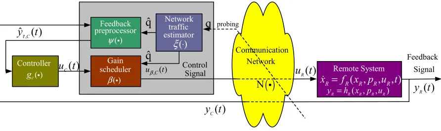
The basic components of GSM, shown in Figure 2, are as follows [15].

1) Network Traffic Estimator: The function of the network traffic estimator

is to estimate the current network conditions. It monitors a probing packet to

find the roundtrip network measurements that are characterized by q. The

variable q is then used by the feedback preprocessor and the gain scheduler to

estimate the current network delays.

2) Feedback Preprocessor: The function of the feedback preprocessor is to

gather the sensor data of the remote system and perform any functions on the

data before passing it to the controller. These functions can include filtering

noise or predicting the state of the remote system.

3) Gain Scheduler: The function of the gain scheduler is to modify the

controller’s output with respect to the current network conditions

(16)

( ) R u t ( ) R y t ( ) C y t ( ) ξ ⋅ ( , , , )

R R R R R

x =f x p u t

( , , )

R R R R R

y =h x p u q

( )

N i Network traffic estimator Control Signal probing Communication Network Remote System Feedback Signal ˆq ˆq

,C( ) u_β t

Feedback preprocessor ( ) ψ i ( ) C u t , ˆ

ˆ ( )C y t_τ

Controller ( ) c g i ( ) β i Gain scheduler

Figure 2. Structure of GSM.

The GSM methodology is adapted to the particular system of interest. In this thesis,

GSM is applied on a networked PI controller for a DC motor.

2-2. Optimal stochastic methodology

The optimal stochastic control methodology treats a networked control system with

random network delays as a Linear Quadratic Gaussian (LQG) problem. This method was

first proposed by Nilsson [4]. To control the system, the methodology assumes that

sc ca _T

τ +τ < , in addition to the previous assumptions. Without this condition, the control

signals could arrive at the actuator out of order, making analysis much more difficult. In

addition, if this assumption is violated, the method cannot guarantee system performance.

The system dynamics are assumed to be linear and can be described by:

( ) ( ) ( ) ( )

( ) ( ) ( )

x t Ax t Bu t v t

y t Cx t w t

= + +

= + , (1)

where ( )_{x t} _∈_Rn _{, ( )}_{u t} _∈_Rm_{, and ( ), ( )}_{v t w t} _∈_Rn _._A _and_B_{are matrices of appropriate}

(17)

noises with zero means [4]. This system can be discretized into kT sampling periods

resulting with the following dynamics:

0 1

( 1) ( ) ( , ) ( ) ( , ) ( 1) ( )

( ) ( ) ( )

sc ca sc ca

x k x k u k u k v k

y k+ = Φ=Cx k +w k+ Γ τ τ + Γ τ τ − + ,(2)

where

0 ₀

1

( , ) ( )

( , ) ( 1)

sc ca k k sc ca k k AT T

sc ca As

T

sc ca As

T e

u k e dsB

−τ −τ −τ −τ Φ = Γ τ τ = Γ τ τ − =

∫

, (3)

and _τsc_{is the network delay from the plant output (sensor) to the controller;}_τca_{is the}

network delay from the controller to the plant input (actuator), and T is the sampling rate of

the sensor [11].

The goal of the optimal stochastic method is to solve the control problem by

minimizing the cost function in the case that full state information is available.

{

}

1

0 ( ) ( ) ( ) ( ) ( ) ( ) ( ) T N T N k

x k x k

J k E x N Q x N E Q

u k u k

− =  _ _ _ _   = +  _ _ _ _       

∑



, (4)

where E

{ }

• is the expected value, and Q_N and Q are weighting matrices. The optimal

control law that minimizes the cost function is:

* *

* 1

( sc) k k k x u K u τ −   = − _ _

 , (5)

where _K*

is the optimal gain matrix after solving the formulated LQG problem [4].

In practice, a table for _K_{[0, ]}(_τsc)

∞ , where K[0, ]∞

( )

• is the optimal gain matrix for

(18)

interpolated from the tabular values in real-time. This is done because of the calculation

intensive process of finding *₍ sc₎

k

K τ .

This method can be simplified into a suboptimal method that has been shown to give

results close to the optimal method but uses less calculations during runtime [11]. The

control law for this method is given by:

1

[ p p] k

k k k

k

x

u K

u ₋

 

= − Φ Γ _ _

 , (6)

where

( )

0

sc ca

k k

sc ca

k k

A E

p k

E

p As

k

e

e dsB

τ τ

+

Φ =

Γ =

∫

. (7)

ca k

Eτ _{is the expected value of}_τca_._K_{is the optimal LQG gain found from the system without}

delay. Thus the non-delay gain, K, is modified by a matrix containing the delay information

for the current step and a prediction of the delay to be experienced from the controller back

to the plant. This operation can be seen as a prediction from the state estimate at the current

time, kT, to a state estimate when the control signal is applied at the plant [11]. This is an

alternative to having the delay information embedded in the K gain matrix. This approach

will be used for this thesis because of its near optimal performance and reduced calculation

(19)

2-3. Queuing methodology

The purpose of adding queues into a networked control system is to reshape the

random time delays into deterministic delays. As an effect, the system becomes

time-invariant. One such method is proposed by Luck and Ray [3, 12]. They propose to use an

observer to estimate the plant states and a predictor to compute the predictive control. The

past measurement data and the control data are stored in a First-In-First-Out (FIFO) queue,

defined as Q₁ and Q₂ of sizes r and α , respectively. The structure of a network control

system utilizing the queuing methodology is shown in Figure 3 [1].

r 1 Q α

2

Q x k( − +α 1) x k r( + )

( ) u k r+ ( )

Z k

( )

y k u k( )

sc

τ

ca

Controller

Plant

Sensor Actuator Predictor Observer

Network

Figure 3. Configuration of networked control system utilizing queuing methodology.

The steps for applying this methodology are listed below [1]:

z Using the set of past measurements Z k( )=

{

y k( −φ), (y k− −φ 1,...

}

(20)

z The predictor uses ˆ(x k− +α 1) to predict the future state ˆ(x k r+ ).

z The controller computes the predictive control u k r( + =) K x k r( (ˆ + )),

where K is the controller gain, and then sends (u k r+ ) to be stored in

1

Q .

The model of the plant must be very precise since the performance of the observer

and predictor depend on it. For a closed-loop NBC system, the various components are

defined below.

Plant model:

1 ,

k k k

x₊ = Ax +Bu y_k =Cx_k; (8)

Observer model:

1|1 |1 ( |1);

k k k k k k

z ₊ =Az +Bu +L y −Cz (9)

δ-step predictor:

1| | 1

k k k

z ₊_δ =Az _δ₋ +Bu for δ ≥2; (10)

Predictive control:

|

k k k

(21)

where z_k_|_δ :=xˆ_{k k}_| ₋_δ is the estimation of x_k given the measurement history

{

, 1, 2,

}

k k k k

Z ₋_δ = Z ₋_δ Z _{− −}_δ Z _{− −}_δ … , {A,B,C} are the realization of the plant system, and the

estimation error:

|1

k k k

e = −x z . (12)

k

Γ and L_k_{represent the proper controller and observer gains, respectively.}δ represents the

number of sample times in a given delay time, or

sc ca T

τ τ

δ = + . (13)

Then, the closed loop system equation can be expressed as

1

1 0

k k k k k

k k k

x A B B x

e _δ A L C e_δ _δ

+ − + − − + Γ − Γ Λ       =    ₋   

     , (14)

where 1 1 1 1 1 1 1 1 1 ( ) : ( ) k j j i i

k k k j

i j

A L C

A L C A L C

I δ δ δ δ δ − + − − − − − − − − + − − −  − +    _ _  Λ =  × −       

∏

if if 2 0 2. δ δ ≥ ≤ < (15)

and the plant model is assumed to be exact [3]. Proof of this proposition can also be found in

[3].

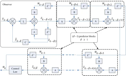
The schematic diagram of a δ -step delay compensation algorithm is shown in Figure

4, where δ represents the delay length in terms of sampling time steps. The lengths of the

(22)

1

k

u _{− +}_δ

2|2

k z _{− +}_δ

2

k

u _{− +}_δ

3|3

k z _{− +}_δ

3

k

u _{− +}_δ

1

k

u ₋

4|4

k z _{− +}_δ

| k z _δ k u + + ++ + + + + k

y ₋_δ

ˆ_k

y ₋_δ

k

u ₋_δ

|1

k z ₋_δ

1|1

k z _{− +}_δ

+ + + + + 1 δ ≥

(δ−1) predictor blocks A

A A

B B B

B B

L

C

-1

Z _Z-1 _Z-1

-1 Z -1 Z -1 Z Control Law Observer

Figure 4. Delay compensation algorithm with predictor blocks.

If _τsc₌_τca ₌_δ_{, then the sensor data received at the controller at time}_k_{has already}

experienced a one time step delay, _τsc_{. That is, it was generated at time (}_{t k}₋₁₎_._{In addition,}

the controller’s gain must also be delivered through the network experiencing another one

step delay, _τca _{. This will result in the control signal being received at the plant at}

timet k( +1). Therefore, the controller must estimate the plant state for the timet k( +1) at

time k so that it can send u k( +1) through the network to be the correct input, u k( ), for the

plant at t k( +1) . This scenario describes a δ =2 compensation algorithm. Figure 5

(23)

sc

τ

_τ

ca

( 1)

y k− u k( +1)

( 1)

t k+

( 1)

t k− t k( )

( )

t k

Plant

Controller

y(k) estimated, y(k+1) estimated, then used to generate u(k+1)

Figure 5 Timing diagram for _τsc ₌_τca ₌_δ_.

As mentioned before, the performance of the methodology depends greatly on the

accuracy of the model and observer. This structure allows for variable delays as long as the

following constraints are met: (1) _τsc₊_τca ₌_{known constant, (2) the sensor and controller}

sampling instants are synchronized with no time skew [3].

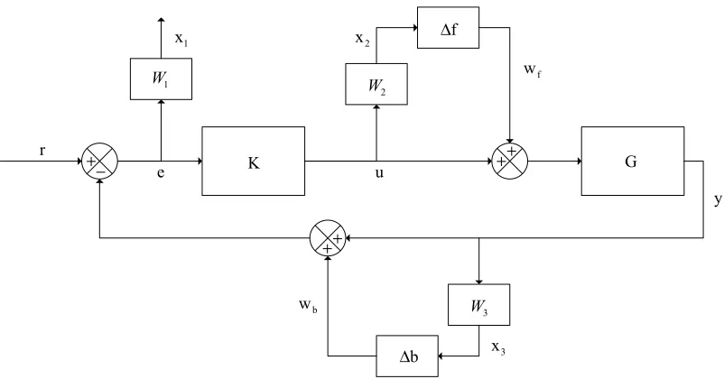
2-4. Robust Control

The robust control methodology models the two network delays, _τsc_and_τca_{, as}

simultaneous multiplicative perturbations. Using H_∞ and µ -synthesis, the perturbations

represent the modeling uncertainties associated with the network delays. The feedback

control system can be modeled in the frequency domain. The purpose of robust control is to

(24)

1 W

2 W

3 W 1

x x2

3

x u

y e

r

f

w

b

w

K G

b

∆

f

∆

+

++

++ −

Figure 6. Controller-Plant Modeling with Network Delays.

The controller-plant model with network delays as perturbations is shown in Figure 6.

f

∆ and ∆b represent the network delays _τca_and_τsc_{, respectively. The delay uncertainty in}

the frequency domain, given as exponential distribution e−τmax∆s

, where 1− < ∆ <1, can be

approximated using a modified Pade approximation with ∆ complex [17]:

max max

max

1 1 ( )

1 2

s s

e W s

s

τ τ

τ

− ∆ _{≈ −} _{∆ = +} _∆

+ , (16)

where ∆ ≤1 and

( )

1 3.465

s W s

s

τ τ

=

+ . (17)

Here, ∆ can be either ∆f and ∆b, and τ can be either _τca_and_τsc_{. W(s) is suggested by}

[17] as an appropriate uncertainty weight that covers the uncertain delay. The factor 3.465 is

(25)

Figure 6. W₁ represents the performance weight for the system in Figure 6 and is determined by the error signal. It is presented here as a low-pass filter as suggested from [14]:

1 2

0.9 ( )

0.9

W s

s s

=

+ + . (18)

The problem is solved using the H_∞ and µ-synthesis toolboxes in Matlab [18]. First,

the problem illustrated in Figure 6 must be formulated into the H_∞ framework shown in

Figure 7, where K is the controller gain to be determined by DK iteration during the H_∞

process.

2 3 1

x x x

         

f b

w w r

         

∆

K P

e u

Figure 7. Robust analysis for a general interconnection system.

The matrix, P, contains the interconnection structure. ∆ =diag

[

∆ ∆ ∆f, b p,

]

, where ∆p is a

fictitious uncertainty block used to incorporate the H_∞ performance objective. The

(26)

2 2

3 3 3

1 1 1 1 1

0 0 0

0 0

1 1

f b

x W w

x W G W G w

x W G W W W G r

e G G u

     

     

  ₌   

  − − −       ₋ ₋ ₋   

     

, (19)

where W₁, W₂, and W₃ are the weights discussed previously, G is the plant dynamics, and

f

w and w_b are introduced to represent the inputs to the system when the perturbations are

omitted during the open-loop formulation of the problem and can be seen in Figure 6. The

necessary condition for robust performance, then, is P K, _∞ <1. This is often measured by

the peak µ value, or ( , ) 1µ P K < . Robust control tries to minimize the effect of a

disturbance on the system as seen by the error signal. This performance measure is given by

( , )P K

µ , which is desired to be driven to zero. If ( , ) 0µ P K = , this would indicate that any

size disturbance would have zero effect on the error, hence displaying ideal robust stability.

(27)

CHAPTER 3 CASE STUDY: DC MOTOR

3-1. System Description

The DC motor is governed by the following equations:

1

B

a a w a

w a w

K R

i i e

L L L

K B

i F

J J J

ω

ω ω

= − − +

= − +

, (20)

where e_a is the armature winding input voltage, L is the armature winding inductance, R is

the armature winding resistance, i_a is the armature winding current, K_B is the back EMF

constant, K is the torque constant, J is the moment of inertia of the wheel and rotor, B is the

damping coefficient of the wheel and rotor, ω_w is the angular velocity of the wheel, and F is

the load torque. Table 1 shows the values used during simulation for these constants that

were modified from [10].

Table 1. DC motor parameters.

K = 2.55e-3 N-m/A R = 6.43 Ω

B

K = .255e-3 V-sec/rad L = 28.8e-3 H

B = 0.1e-3 N-m-sec/rad J = 3.53e-6 Kg-m2

The sampling time, T, for the controller is chosen to be 0.1ms. This is to capture the

(28)

4.48 msec

e L R

γ = = . (21)

The load torque is assumed to be zero during the simulations. (20) can be arranged

into the standard state space form shown below:

1

0

b K

R _i

i _L _L

L u b

K

J J ω

ω

−

₋  _ _

  _ _ 

= + 

  _ ₋ _ 

   

  __ __ _ _ . (22)

During the simulations, the plant is considered to be described by (22) that is sampled

every kT seconds. The plant output is assumed to be fully observable.

A PI controller will be used that has been tuned for nominal performance in the

non-delay case for the controller of the system. The control voltage, e_a, is assumed to be

bounded by ±12 volts. The optimal PI gains for the non-delay case are determined by the

root locus approach and must satisfy the following design requirements:

Relative damping ratio: 0.707;

Percentage overshoot: . . 5%;

Settling time: 0.0321sec;

Rise time: 0.014sec;

s r

P O t

t

ζ

• =

• ≤

(23)

Using the above requirements, ₍ *_, *_{) (25.572,0.995)}

I P

K K = will satisfy the conditions above.

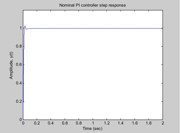
This will be used as the baseline performance to compare to. The reference speed is set to

( ) 1

r k = rad/sec. The nominal performance of the PI controller with *

I I

K =K and *

P P

K =K

(29)

0 0.2 0.4 0.6 0.8 1 1.2 1.4 1.6 1.8 2 0 0.2 0.4 0.6 0.8 1 Time (sec) A m pl itud e, y (t )

Nominal PI controller step response

Figure 8. Nominal PI controller step response with ₍ *_, *_{) (25.572,0.995)}

I P

K K = .

3-2. Performance Characterization

In order to characterize the performance of each methodology, the following

performance measure is adopted [5, 15]:

1 1 2 2 3 3

J =w J +w J +w J , (24)

2 0 0 1 0 ( ) , 0,

MSE MSE MSE MSE

J

MSE MSE

 − >

=

≤

 , (25)

2

0 0

2

0

( . . . . ) , . . . .

0, . . . .

P O P O P O P O

J

P O P O

 − >

= _≤

 , (26)

2 0 0 3 0 ( ) , 0,

r r r r

r r

t t t t

J

t t

 − >

= _≤

 , (27)

(30)

is the mean-squared error, MSE₀ is the nominal mean-squared error, P O. .₀ is the nominal

percentage overshoot, t_r₀ is the nominal rise time. The weights w w₁, ₂,and w₃ specify the

relative significance of J J₁, ₂, and J₃, respectively, on the overall system performance.

The error, ( )e k =y k( )−r k( ), is computed by sampling ( )y t every kT time instant. The costs

1, 2,

J J and J₃ penalize any degradation in performance from the nominal case. The

nominal performance meets the design specification such that MSE₀ =0.003405,P O. .₀ =5%,

and t_r₀ =0.014. MSE₀ is determined by simulation or by experiment. In the nominal

non-delay case, the cost function in (24) will equal zero. J₁ penalizes tracking error. J₂

penalizes higher overshoot. J₃ penalizes the slower response time. The weightsw w₁, ₂,and

3

w are found by simulation using the GSM method with β =

[ ]

0, 2 and no delay with the

following equation:

1

1, 2,3 max( ) min( )

i

i i

w for i

J J

= =

− . (29)

When 1β = , the nominal gain is applied to the system and therefore the cost J =0.

Therefore, min( ) 0J_i = for i=1, 2,3 and (29) reduces to

1

1, 2,3 max( )

i

w for i

J

= = . (30)

For the DC motor parameters listed in Table 1, w₁ =17.4572 , w₂ =0.0066771, and

3 0.8777

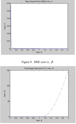
w = . The cost graphs for J J₁, ₂, and J₃ for β =

[ ]

0, 2 are shown in Figure 9,

(31)

0 0.2 0.4 0.6 0.8 1 1.2 1.4 1.6 1.8 2 0

0.01 0.02 0.03 0.04 0.05 0.06

Gain, B

Cos

t,

J

1

Mean Squared Error (MSE) cost, J1

Figure 9. MSE cost vs. β.

0 0.2 0.4 0.6 0.8 1 1.2 1.4 1.6 1.8 2

0 50 100 150

Gain, B

C

os

t, J

2

Percentage Overshoot (P.O.) cost, J2

(32)

0 0.2 0.4 0.6 0.8 1 1.2 1.4 1.6 1.8 2 0

0.2 0.4 0.6 0.8 1 1.2 1.4

Gain, B

Cos

t,

J

3

Rise Time (t.r.) cost, J3

(33)

3-3. Network Delay

Each methodology has its specific way of modeling the network delay experienced on

the system. In general, network delay will be modeled as an exponential distribution unless

otherwise noted. The generalized exponential distribution to describe IP network delays is as

follows [15]:

[ ]

1 ( ) ,

0,

e P

τ η φ _{τ η}

φ τ

τ η

− −

 _≥



=

 _<



, (31)

where η is the minimum transportation delay of the application. The expected value of the

RTT delay is ( )Eτ = +φ η with variance, _σ2 ₌_φ2_{, and median,}_η_..

Keeping in mind the DC motor’s time constant denoted in (21),

[0.0001, 0.001, 0.005, 0.01,0.05,0.1]

η = has been chosen to simulate the RTT IP-network

delay and be representative of a variety of minimum network transportation delays possibly

experienced. The first two delays should have smaller effects on the system performance as

they are less than 0.5γ_e found in (21) (i.e., can capture the electrical dynamics of the DC

motor), while the larger delays should cause more rapid system degradation. A typical

(34)

0 0.2 0.4 0.6 0.8 1 x 10-3 0

1000 2000 3000 4000 5000 6000 7000 8000 9000 10000

Time (sec)

De

ns

ity

Histogram: 0.0001 RTT Network Delay

mean = 0.0001

(35)

CHAPTER 4 SIMULATION RESULTS

For all simulations, the final time, t_f, is 2 seconds, with a sampling time, T, of 0.0001

seconds. Matlab 7.0 was used to run the simulations. The following sections will present the

results for each of the four methods in alphabetical order when applied to the DC motor

model described previously. Afterwards, the performance of the methods will be

characterized with respect to the other models.

4-1. Gain scheduling middleware (GSM)

4.1.1 DC Motor Application

GSM will be applied on the networked PI controller for a DC motor. The transfer

function of the PI controller is given as:

( )

( ) p C

c

K s z G s

s +

= , (32)

where z_C =K K_I _P is a constant. The optimal PI gains for the non-delay case are determined

by the root locus approach and satisfy the following design requirements as shown in (23).

* *

(K K_I, _P) (25.572,0.995)= will satisfy the requirements. With this choice of gains,

25.7

C

z = . The response at this gain setting will be the baseline performance to compare to.

(36)

Letβ be the gain scheduling parameter that will modify the gain. In this case, β will

modify the PI gain in the following way:

( )

( ) P C

c

K s z G s

s

β

β = + . (33)

By keeping z_C a constant, the optimization of β becomes a one-dimensional problem rather

than a two-dimensional problem where K_I and K_P were allowed to vary independently.

The optimalβ for a given delay is found by minimizing the cost function given in

(24). This can be done for several expected delays. The cost, J, from this optimization is

shown in Figure 13 and Figure 14. GSM can then use a look-up table to select the

appropriateβ for the delay measured by the network traffic estimator. Table 2 shows the

optimalβ for the delay set, η, presented previously using the cost function in (24).

Table 2. Optimal β gains for various time delays.

Delay Time (sec) 0.0001 0.001 0.005 0.01 0.05 0.1

(37)

0 0.2 0.4 0.6 0.8 1 1.2 0

0.01 0.02 0.03 0.04 0.05 0.06

Gain, B

C

os

t, J

Cost J from optimization

delay = 0.0001 delay = 0.001 delay = 0.005

Figure 13. Cost vs. β for η=[0.0001,0.001,0.005] network delays.

0 0.05 0.1 0.15 0.2 0.25 0.3 0.35 0.4

0 0.01 0.02 0.03 0.04 0.05 0.06 0.07 0.08 0.09 0.1

Gain, B

C

ost, J

Cost J from optimization

delay = 0.01 delay = 0.05 delay = 0.1

(38)

4.1.2 Results

The optimalβ decreases as the network delay increases. This lowers the system

response time in response to an increase in network delay to ensure stable operation. The

cost, J, is more sensitive to variations in delay as the delay time increases, shown in Figure

13 and Figure 14 as the width of the cost curve decreases with higher delays. The step

response of the DC motor plant with the nominal PI controller only, and with GSM

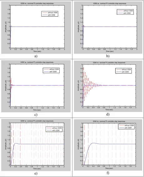
implemented, in the presence of the set of network delays, η, is shown in Figure 15.

As the network delay increases past 0.01 sec, the controller is unable to stabilize the

system. Using the optimal β value found offline, the GSM method is able to maintain

system stability at the cost of slower response time. The responses with GSM have fewer

oscillations as they approach the reference value. In all cases, the GSM method is able to

stabilize to the reference value, while the nominal PI controller fails to stabilize for the 0.05

and 0.01 second delays.

Table 3 shows the performance comparison between the nominal case and all four

methods. For all delays, GSM equals or outperforms the uncompensated nominal PI

(39)

0 0.2 0.4 0.6 0.8 1 1.2 1.4 1.6 1.8 2 0 0.2 0.4 0.6 0.8 1 1.2 1.4 1.6 1.8

2 GSM vs. nominal PI controller step responses

Time (sec) A m pl itud e, y (t ) without GSM with GSM a)

0 0.2 0.4 0.6 0.8 1 1.2 1.4 1.6 1.8 2 0 0.2 0.4 0.6 0.8 1 1.2 1.4 1.6 1.8

Time (sec) A m pl itud e, y (t ) without GSM with GSM b)

0 0.2 0.4 0.6 0.8 1 1.2 1.4 1.6 1.8 2 0 0.2 0.4 0.6 0.8 1 1.2 1.4 1.6 1.8

Time (sec) A m pl itu de, y (t ) without GSM with GSM c)

0 0.2 0.4 0.6 0.8 1 1.2 1.4 1.6 1.8 2 0 0.2 0.4 0.6 0.8 1 1.2 1.4 1.6 1.8

Time (sec) A m pl itud e, y (t ) without GSM with GSM d)

0 0.2 0.4 0.6 0.8 1 1.2 1.4 1.6 1.8 2 0 0.2 0.4 0.6 0.8 1 1.2 1.4 1.6 1.8

Time (sec) A m pl itu de, y (t ) without GSM with GSM e)

0 0.2 0.4 0.6 0.8 1 1.2 1.4 1.6 1.8 2 0 0.2 0.4 0.6 0.8 1 1.2 1.4 1.6 1.8 2

GSM vs. nominal PI controller step responses

Time (sec) A m pl itud e, y (t ) without GSM with GSM f)

Figure 15. Nominal PI controller vs. GSM step responses for a) η=0.0001 b) η=0.001 c)

0.005

(40)

4-2. Optimal stochastic method

4.2.1 DC motor application

The constraining assumption of the optimal stochastic method is that _τsc₊_τca _<_T_.

Since _τsc_and_τca_{must be measured and used in the calculation of the LQG gain, timestamps}

are added to each packet in order to measure the delay experienced. The standard LQG

problem regulates the plant output around zero. In this case, it is desired for the system to

track a reference input. In order to formulate the regulator as a tracking problem, the output,

( )

y k , must be compared to the reference signal, ( )r k . The goal is then to drive the error

between the output and the reference to zero. A common practice is to add an integrator to

the error signal, ( )e k =y k( )−r k( ), to drive it to zero [19]. The reformulated LQG problem

can then be solved using the Matlab Control System toolbox.

For the DC motor, the LQG control objective is to minimize the cost function:

( ) ( T T 2 T )

J u x Qx u Ru x Nu dt

∞

=

_∫

+ + , (34)

Table 3. Performance comparison of four methodologies for different RTT network delays.

Delay Time (sec) Control

Scheme 0.0001 0.001 0.005 0.01 0.05 0.1

Nominal 4.68E-09 0.016480118 6.183768417 43.88451303 3.95E+57 2.65E+45

GSM 0 1.53E-06 1.45E-04 6.74E-04 0.019338165 0.079725567

Robust 0.247174844 0.001999007 0.016218814 0.037692917 0.505627477 6.074238664

LQG 0 0.417990105 30.57058632 4.01E+02 1.05E+05 3.61E+07

(41)

where (1 6,10,10)Q diag e= , R=1, and N =0, for the augmented plant description with the

integrator on the error signal, where the states are defined as x=

{

e i, ,ω

}

T. Q, R, and N are

determined experimentally by finding the LQR gain whose performance best mirrors that of

the PI controller during a non-delay case trial. This puts the largest penalty on the error

while also keeping the control values within the acceptable limits of ±12V . The white

noises v t( ) and w t( ) are assumed to be zero in order to properly compare the performance of

each methodology. The assumption is that the network delay is the dominating factor of the

system performance and stability.

Using the problem formulation above, the LQG controller is designed without taking

any delays into account. This yields a gain K = −

[

1000,12.404, 7.2913

]

.

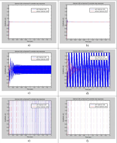
4.2.2 Results

Table 3 shows the comparison of (24) between the nominal PI controller and the LQG

controller. The step response comparisons are shown for the LQG controller versus the

nominal PI controller in Figure 16. It performs very well for 0.0001 sec delay since the

major assumption of _τsc₊_τca _<_T_{is met. Notice that it does manage to lower the cost at the}

highest delays of 0.05 and 0.1 seconds even though the tracking performance fails to stabilize.

The performance degrades faster than the nominal case since T is held constant at 0.0001,

(42)

0 0.2 0.4 0.6 0.8 1 1.2 1.4 1.6 1.8 2 0 0.2 0.4 0.6 0.8 1 1.2 1.4 1.6 1.8 2

Optimal LQG vs Nominal PI controller step responses

Time (sec) A m pl itude, y (t )

with Optimal LQG without Optimal LGQ

a)

0 0.2 0.4 0.6 0.8 1 1.2 1.4 1.6 1.8 2 0 0.2 0.4 0.6 0.8 1 1.2 1.4 1.6 1.8

2 Optimal LQG vs Nominal PI controller step responses

Time (sec) A m pl itud e, y (t )

b)

0 0.2 0.4 0.6 0.8 1 1.2 1.4 1.6 1.8 2 0 0.2 0.4 0.6 0.8 1 1.2 1.4 1.6 1.8

c)

0 0.2 0.4 0.6 0.8 1 1.2 1.4 1.6 1.8 2 0 0.2 0.4 0.6 0.8 1 1.2 1.4 1.6 1.8

Time (sec) A m pl itu de, y (t )

d)

0 0.2 0.4 0.6 0.8 1 1.2 1.4 1.6 1.8 2 0 0.2 0.4 0.6 0.8 1 1.2 1.4 1.6 1.8 2

e)

0 0.2 0.4 0.6 0.8 1 1.2 1.4 1.6 1.8 2 0 0.2 0.4 0.6 0.8 1 1.2 1.4 1.6 1.8 2

Time (sec) A m pl itud e, y (t )

f)

Figure 16. Nominal PI controller vs. Optimal stochastic method step responses for

(43)

4-3. Queuing methodology

Since full state information is available, the observer block shown in Figure 3 and

Figure 4 is omitted. Thus for a δ -step delay, where δ is the delay measured in terms of the

number of sample times, δ predictor blocks will be needed. For example, the 0.001 RTT

delay will require 0.001/0.0001 or 10 predictor blocks. It should be noted that the queuing

method depends on the accuracy of the model and observer. Since the model is accurate and

no observer is used, we should expect to see very good results.

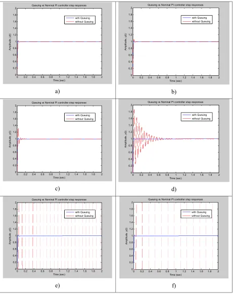
4.3.2 Results

The results of the queuing method versus the nominal PI controller are shown in

Figure 17. Note that the responses for each delay are identical. This is because of the perfect

model and full state information. Table 3 shows the costs associated with the queuing

methodology for the different delays. As noted before, because of the perfect model

accuracy, the predictor block is able to predict the states perfectly regardless of the delay.

However, the queue length increases as the delay increases, as shown in Table 4. This could

provide difficulties when implementing the queuing methodology for a real-time application

since the computation time could be significant. The queuing methodology works well when

the delay is bounded by a constant and the plant model is known. Also, it is more feasible

for time sensitive applications when the sample time is close to the delay time to limit the

(44)

Table 4. Queue lengths for various delays.

Delay (sec) Queue Length

0.0001 1

0.001 10

0.005 50

0.01 100

0.05 500

(45)

0 0.2 0.4 0.6 0.8 1 1.2 1.4 1.6 1.8 2 0 0.2 0.4 0.6 0.8 1 1.2 1.4 1.6 1.8 2 Time (sec) A m pl itude, y (t )

Queuing vs Nominal PI controller step responses

with Queuing without Queuing

a)

0 0.2 0.4 0.6 0.8 1 1.2 1.4 1.6 1.8 2 0 0.2 0.4 0.6 0.8 1 1.2 1.4 1.6 1.8 2 Time (sec) A m pl itud e, y (t )

b)

c)

0 0.2 0.4 0.6 0.8 1 1.2 1.4 1.6 1.8 2 0 0.2 0.4 0.6 0.8 1 1.2 1.4 1.6 1.8 2 Time (sec) A m pl itu de, y (t )

d)

e)

(46)

4-4. Robust control methodology

G represents the plant dynamics and are given for the DC motor in (22). These will

be used to form the interconnection matrix P. By experimentation, the performance weight,

1

W , was found to be

1 2

25 ( )

20 1

W s

s s

=

+ + . (35)

This gives satisfactory performance for all delays. W₂ and W₃ are given in (17).

Next the system is analyzed using the dkitgui tool in Matlab. This tool uses DK

iteration to generate controllers for the system and analyze the robustness using µ -synthesis.

For the DC motor, the frequency range 0.001 to 1000 with 1000 points was used. The

uncertainty structure is a 2x2 matrix. Eight iterations were completed for each delay time,

generating eight controllers. Each one was tested for optimal performance based on the

performance measure in (24). The best one was chosen for the final trials. The controller

chosen also had the lowest peak µ value given by the dkitgui tool. A lower µ value

indicates a smaller effect of a disturbance (i.e. network delay) on the system.

Overall, the robust methodology does a great job as compensating for network delay.

The major benefit is that the controller does not need a priori knowledge of the network

delays, nor does it need the past delay measurements as many of the other methods do. It

does, however, require that the weights be carefully set such that they cover the uncertain

(47)

4.4.2 Results

The optimal robust controller for each delay is shown in Table 5 . The number

indicates during which iteration the optimal performance, or lowest cost, was achieved. Thus

for the first delay of 0.0001 sec, the 4th D-K iteration controller achieved the best results and

was, therefore, used for the final simulation runs. In all cases but η =0.1sec, the controller

with the lowest peak µ value produced the best performance. The peak µ values for each

of the eight controllers generated for each delay time can be found in Table 6.

Table 5. Optimal robust controller for each delay.

Delay time

(sec) 0.0001 0.001 0.005 0.01 0.05 0.1

Controller

number 4 7 8 7 3 1

Table 6. Peak µ values for controller generated during each DK iteration.

Optimal controller values are shown in italic.

D-K iteration number Delay

time

(sec) 1 2 3 4 5 6 7 8

0.0001 0.029 0.012 0.013 0.012 0.012 0.013 0.018 0.012

0.001 0.111 0.046 0.044 0.046 0.044 0.044 0.044 0.044

0.005 0.317 0.109 0.108 0.106 0.123 0.111 0.109 0.107

0.01 0.516 0.163 0.155 0.157 0.155 0.157 0.155 0.157

0.05 1.9963 0.641 0.641 1.1826 1.9359 0.941 0.934 0.975

(48)

The step responses comparing the robust control method and the nominal PI

controller are shown in Figure 18. The cost for the 0.0001 sec delay is larger than the 0.001

delay because the D-K iteration tries to optimize its control to the H_∞ performance measure

that differs from the one given in (24). Aside from that result, the cost increases as the delay

time increases, and on the whole, the robust method compensates for the delay as shown by

(49)

0 0.2 0.4 0.6 0.8 1 1.2 1.4 1.6 1.8 2 -0.5 0 0.5 1 1.5 2 Time (sec) A m pl itude, y (t )

Robust vs. Nominal PI controller step response results

with Robust without Robust

a)

0 0.2 0.4 0.6 0.8 1 1.2 1.4 1.6 1.8 2 -0.5 0 0.5 1 1.5 2 Time (sec) A m pl itud e, y (t )

b)

c)

0 0.2 0.4 0.6 0.8 1 1.2 1.4 1.6 1.8 2 -0.5 0 0.5 1 1.5 2 Time (sec) A m pl itu de, y (t )

d)

e)

0 0.2 0.4 0.6 0.8 1 1.2 1.4 1.6 1.8 2 -0.5 0 0.5 1 1.5 2 Time (sec) A m pl itud e, y (t )

f)

(50)

CHAPTER 5 NOISE

The previous results were conducted under ideal conditions. The performance of

each method was also investigated under noisy conditions. Noise was introduced into the

control loop at the sensor measurement to simulate modeling errors (both state and

measurement). Figure 19 shows how the noise, w k( ), is introduced into the system. The

noise is Gaussian white noise with the zero mean and a given variance, _{v k}_{( )}₌_G_{( ,}_{µ σ}2₎_.

The mean, µ, is set to zero and the variance, _σ2_{, was chosen so that the distribution effected}

between 0 and 10% of the final reference value of 1 rad/sec. This was determined by

3σ

Ψ = , where Ψ stands for the noise level with respect to the final value, and σ is the

standard deviation. 3σ was chosen as it accounts for 99.7% of a normal distribution. Thus

for ψ∈

{

0.5% 1% 2% 5% 10%

}

, the variance used is

2 2.7778e-06,1.1111e-05, 4.4444e-05,

0.00027778,0.0011111

σ ∈ 

 . (36)

The distributions of the variances are shown in Figure 20. The performance is measured with

the same performance measure described earlier in (24). With noise added, the typical step

(51)

K G r

e u

y +

- τca ++

sc

τ

Figure 19. Noise, w k( ) introduced into the control loop.

-0.1 -0.05 0 0.05 0.1 0

50 100 150 200

Data

De

ns

ity

Random Noise Distributions

0.5% 1% 2% 5% 10%

Figure 20. Noise distributions.

0 0.2 0.4 0.6 0.8 1 1.2 1.4 1.6 1.8 2

-0.2 0 0.2 0.4 0.6 0.8 1 1.2

Time (sec)

A

ngu

la

r V

el

oc

ity

(

rad/

se

c)

(52)

It is expected that the introduction of noise will decrease the performance of the

system. As the noise increases, the performance should decrease which will be indicated by

a higher cost measured by (24). Figure 22 shows the results for each method with respect to

RTT delay and the noise level.

In general, as the delay and noise increase, so does the cost J. The queuing and GSM

methods have the lowest cost with respect to noise or network delay.

0

5

10

10-4 10-3

10-2 10-1

10-20 10-15 10-10 10-5 100 105 1010

% Noise level (linear) Network delay and noise level performance comparison

RTT Delay time - sec (log)

C

ost

, J (

lo

g)

Queuing Robust LQG GSM

Figure 22. Performance comparison with noise.

5-1. GSM

Figure 23 shows the performance of the GSM methodology with noise. For small

delays (i.e. under 0.01 sec), the noise had a larger effect on the performance than for larger

(53)

than the delay, as shown by cost values very similar regardless of the noise level. However,

the total cost at even the worse condition is still much lower than the nominal PI controller.

Table 7 gives the cost, J, for each trial.

0 2

4 6

8 10

10-4 10-3

10-2 10-1

10-20 10-15 10-10 10-5 100

% Noise Level (Linear) GSM Network delay and noise level performance comparison

C

ost, J

(

lo

g)

Figure 23. GSM noise vs. delay performance.

Table 7. GSM noise results.

Noise level

Delay 0% 0.5% 1% 2% 5% 10%

0.0001 0 0 0 0 0 0

0.001 1.53E-06 3.0506E-06 1.1818E-05 5.2972E-05 3.6717E-04 1.5607E-03

0.005 1.45E-04 1.4359E-04 1.4355E-04 1.4347E-04 2.0716E-04 6.4517E-04

0.01 6.74E-04 6.7411E-04 6.7402E-04 6.7387E-04 6.713E-04 6.6879E-4

(54)

5-2. Optimal stochastic method

Figure 24 presents the performance of the optimal stochastic method with noise. As with the

GSM method, the noise effect is more apparent at low delays, 0.001 sec and smaller, than at

higher delays. This is partly due to the noisy results of the optimal method even without

noise, as shown in Figure 16. Those results are due to the fact that _τsc₊_τca _≤/_T_{, where}

0.0001sec

T = in this case. Therefore, additional noise will have little effect on the

performance of the optimal methodology. However, for where _τsc₊_τca _≤_T _{holds true,}

increased noise causes an increase in cost which indicates a decrease in performance. Table

8 gives the cost, J, for each trial.

0 2

4 6

8 10

10-4 10-3 10-2 10-1 10-20 10-10 100 1010

% Noise Level (linear) LQG Network delay and noise level performance comparison

C

ost, J (

lo

g)

(55)

Table 8. Optimal method noise results.

Noise level

Delay 0% 0.5% 1% 2% 5% 10%

0.0001 0 0 0 0 0.028246 0.55458

0.001 0.41799 0.44648 0.49424 0.59705 0.96373 1.769

0.005 30.5706 29.902 30.972 31.712 33.688 24.951

0.01 401.5 427.79 388.85 358.34 383.15 398.74

0.05 1.05E+05 1.0497E+05 1.0506E+05 1.0474E+05 1.0507E+05 1.0528E+05

0.1 3.61E+07 3.6069e+07 3.6068e+07 3.6066e+07 3.606e+07 3.6049e+07

5-3. Queuing method

Figure 25 presents the queuing method’s results with respect to noise levels and

network delay. As mentioned earlier, because of the high accuracy of the model, the queuing

method is able to accurately predict the plant’s state regardless of the delay length. Thus an

increase in delay has no effect on the performance, as the cost does not rise. However, as

noise is introduced, the inputs to the predictor blocks are no longer accurate. This inaccurate

prediction results in an increase in the cost as the noise level increases. Therefore, system

performance degrades as noise levels increase. Similar to the GSM method, the total cost of

the queuing method at the worst condition is still low compared to the nominal PI controller.

(56)

0 2

4 6

8 10

10-4 10-3 10-2 10-1 10-20 10-15 10-10 10-5 100

% Noise level (linear) Queuing Network delay and noise level performance comparison

C

os

t, J

(

lo

g)

Figure 25. Queuing method noise vs. delay performance.

Table 9. Queuing method noise results.

Noise level

Delay 0% 0.5% 1% 2% 5% 10%

0.0001 0 0 1.1135E-09 3.3109E-08 0.018747 0.14272

0.001 0 0 1.2453E-09 3.4573E-08 0.019001 0.12165

0.005 0 0 1.4832E-09 3.7668E-08 0.017853 0.12

0.01 0 0 1.4457E-09 3.7625E-08 0.016157 0.1236

0.05 0 0 1.2905E-09 3.4895E-08 0.017255 0.11824

(57)

5-4. Robust method

Figure 26 shows the performance of the robust methodology for various noise levels

and network delays. Unlike the other methods, regardless of the delay an increase in the

noise level resulted in an increase in the cost, just as an increase in the network delay resulted

in an increase in the cost. Thus, performance degrades as both the network delay and noise

levels increase. However, the increase in the cost, J, at each noise level was less than other

methods as the network delay increased, signifying the methods robustness to disturbances.

Table 10 gives the cost, J, for each trial.

0 2

4 6

8 10

10-4 10-3 10-2 10-1 10-4 10-2 100 102

% Noise level (linear) Robust Network delay and noise level performance comparison

C

ost, J (

lo

g)

(58)

Table 10. Robust methodology noise results.

Noise level

Delay 0% 0.5% 1% 2% 5% 10%

0.0001 0.247174844 0.27621 0.31253 0.38946 0.6814 1.3254

0.001 0.001999007 0.0020004 0.0020107 0.0020259 0.009546 0.35354

0.005 0.016218814 0.015888 0.015803 0.015502 0.018892 0.35448

0.01 0.037692917 0.037065 0.036059 0.034803 0.034417 0.34935

0.05 0.505627477 0.50487 0.50263 0.50045 0.48733 0.83974

(59)

CHAPTER 6 CONCULSION

Four methodologies were investigated for use with real-time applications in a NBC

setting. The simulation results have shown promising results to apply these methodologies

on real-time network-based control systems. The GSM and queuing methods presented the

best performance for various delays and noise levels, as compared to the networked nominal

PI controller. The robust methodology also showed a significant improvement over the

nominal PI controller. The optimal stochastic method showed increased performance over its

limited range set by its delay assumption. Each of the top two performers have certain

drawbacks, namely: GSM has considerable off-line calculations that must be done in order

to schedule the gain for the network traffic conditions, while the queuing method depends

significantly on the plant model’s accuracy. For critical real-time applications, the

appropriate method must be chosen based on the application. All methods have shown the

ability to stabilize the closed loop control system and minimize the detrimental delay effect

in an IP network environment.

6-1. Benefits Table

The purpose of this section is to provide the benefits and drawbacks of the

methodologies so that one may be chosen that best fits the application. Table 11 lists the

pros and cons of each methodology. Gain scheduling middleware is best when the original

Performance Characterization of IP Network-based Control Methodologies for DC Motor Applications.

ABSTRACT

BIOGRAPHY

ACKNOWLEDGMENTS

TABLE OF CONTENTS

LIST OF FIGURES

LIST OF TABLES

CHAPTER 1

INTRODUCTION

τ

τ

CHAPTER 2

BRIEF DESCRIPTION OF FOUR NBC METHODS

( )

∫

∫

{

}

∑

{ }

( )

e

e dsB

Φ =

Γ =

∫

τ

τ

{

}

{

}

∏

∏

∏

τ

τ

[

]

CHAPTER 3

CASE STUDY: DC MOTOR

[ ]

[ ]

[ ]

CHAPTER 4

SIMULATION RESULTS

∫

{

}

[

]

CHAPTER 5

NOISE

{

}

CHAPTER 6

CONCULSION

_τ

_∫