ABSTRACT
GUPTA, SARANSH. ScalaMemAnalysis-MultiLevel: A Compositional Approach to Multi-level Cache Analysis of Compressed Memory Traces. (Under the direction of Dr. Frank Mueller.)
Traditional cache simulators use large trace files or statistical summaries that ignore valuable access pattern details. Analyzing these files is expensive since one needs to constantly update the complete cache state per trace under simulation. In previous work, ScalaMemTrace (SMT) and ScalaMemAnalysis (SMA) were developed. SMT is a tool that records memory traces (load and store instructions) using binary instrumentation and compresses them. SMA exploits these compressed traces to reduce the duration of cache analysis for uniprocessor systems.
© Copyright 2015 by Saransh Gupta
ScalaMemAnalysis-MultiLevel: A Compositional Approach to Multi-level Cache Analysis of Compressed Memory Traces
by Saransh Gupta
A thesis submitted to the Graduate Faculty of North Carolina State University
in partial fulfillment of the requirements for the Degree of
Master of Science
Computer Science
Raleigh, North Carolina
2015
APPROVED BY:
Dr. Nagiza Samatova Dr. Emerson Murphy-Hill
DEDICATION
BIOGRAPHY
ACKNOWLEDGEMENTS
I am deeply indebted to my advisor, Dr. Frank Mueller, for showing confidence in me and his endless guidance during this thesis work. His guidance and feedback kept me on the right track through the course of my thesis. I am also thankful to my committee members, Dr. Nagiza Samatova and Dr. Emerson Murphy-Hill, for discussing and providing useful feedback for this work. I would also like to thank Dr. Xipeng Shen for his feedback on this work.
I am thankful to my colleagues, Xiaoqing Luo, Vishwanathan Chandru, Yasaswini Jyothi, David Fiala, Amir Bahmani and Arash Rezaei, who have supported me in my research work through reviews, discussions and meetings. I am thankful to my roommates Saurabh, Anudeep and Naval, and my friends, Arpit, Amit, Shashank, Snehal, Wageesha and Manasi, for making my life wonderful here in Raleigh.
I am thankful to my friends from JIIT, Rupal, Himanshu, Anshul, Anika, Alekh and Devesh, who have inspired me to do the thing I wanted and pursue my dream. Their endless support was my motivation for pursuing a Masters.
TABLE OF CONTENTS
LIST OF FIGURES . . . vi
Chapter 1 INTRODUCTION . . . 1
1.1 Hypothesis . . . 2
1.2 Contributions . . . 2
1.3 Related Work . . . 3
Chapter 2 BACKGROUND WORK . . . 5
2.1 ScalaMemTrace . . . 5
2.2 ScalaMemAnalysis . . . 6
2.2.1 Assumptions . . . 7
2.2.2 ScalaMemAnalysis Design . . . 7
Chapter 3 SCALAMEMANALYSIS-MULTILEVEL REDESIGN . . . 10
3.1 Design . . . 10
3.1.1 Assumptions . . . 11
3.1.2 Local Cache Tree Structure . . . 12
3.2 Implementation . . . 14
3.2.1 Local Cache Tree’s Miss Pattern Updation Algorithm . . . 14
3.2.2 Miss Pattern Reconstruction Algorithm . . . 16
3.2.3 Regularization . . . 18
Chapter 4 EXPERIMENTATION . . . 19
4.1 Analysis Cost . . . 19
4.2 Accuracy . . . 22
Chapter 5 CONCLUSION . . . 26
Chapter 6 FUTURE WORK . . . 27
BIBLIOGRAPHY . . . 28
APPENDICES . . . 30
Appendix A RSDs AND PRSDs . . . 31
Appendix B MEMORY LATENCY PREDICTIONS . . . 33
LIST OF FIGURES
Figure 2.1 Trace Compression for nested loop using ScalaMemTrace . . . 6
Figure 2.2 Dynamic Pattern Matching for Compressing Memory References. . . 7
Figure 3.1 Workflow Through ScalaMemTrace (SMT), ScalaMemAnalysis (SMA) along with ScalaMemAnalysis-MultiLevel (SMA-ML) redesign. . . 11
Figure 3.2 ScalaMemAnalysis-MultiLevel: Workflow of SMA-ML using the Local Cache Tree (LCT) through an unblocked matrix-multiplication example. . . 13
Figure 4.1 Execution Time Results for Unblocked Matrix Multiplication . . . 20
Figure 4.2 Execution Time Results for Blocked Matrix Multiplication . . . 20
Figure 4.3 Execution Time Results for SPEC Benchmark Suite . . . 21
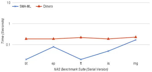
Figure 4.4 Execution Time Results for NAS Benchmark Suite . . . 21
Figure 4.5 L2 Cache Analysis: Accuracy Results for Unblocked Matrix Multiplication . . . 23
Figure 4.6 L2 Cache Analysis: Accuracy Results for Blocked Matrix Multiplication . . . 23
Figure 4.7 L2 Cache Analysis: Accuracy Results for SPEC Benchmark Suite . . . 24
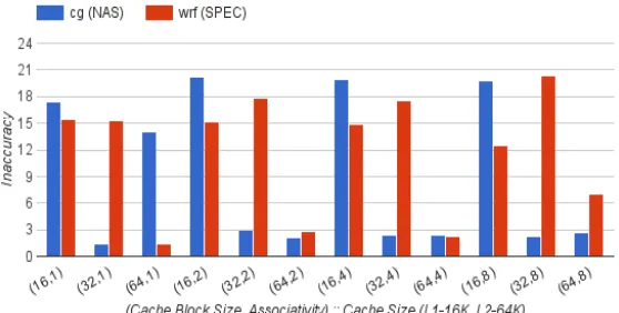
Figure 4.8 L2 Cache Analysis: Accuracy Results for NAS Benchmark Suite . . . 24
Figure B.1 L2 Cache Analysis: Memory Latency Results for SPEC Benchmark Suite . . . . 34
Figure B.2 L2 Cache Analysis: Memory Latency Results for NAS Benchmark Suite . . . 34
CHAPTER
1
INTRODUCTION
Over the past years, the demand for processing has increased exponentially. This has aided advances in supercomputing, accelerators and distributed clusters with shared memory nodes spanning over hundreds of cores. These systems usually keep frequently used data in cache but are constrained by small cache capacity. Since large L1 caches increase the cost of infrastructure, an economical solution is to implement multiple cache levels with slower but larger L2 and L3 caches providing more space. Even commodity computers today use multiple cache levels to exploit spatial and temporal locality. However, these systems still face frequent memory bottlenecks. In order to identify memory bottlenecks and best utilize application data structures, developers may resort to cache simulators.
Understanding or analyzing memory constraints via traditional cache simulation is a cumbersome and time-consuming process. This is because the trace files produced by computers and distributed clusters easily exceed millions of memory references. Cache simulators use such lengthy trace files, containing Gigabytes of data of memory addresses and access types, and maintain complete cache states. The cache states are updated as the trace is processed to compute hit and miss statistics. As an alternative, ScalaMemTrace (SMT) and ScalaMemAnalysis (SMA) were developed to reduce the size of trace files and the analysis overhead in prior work [Bud12; BM14].
1.1. HYPOTHESIS CHAPTER 1. INTRODUCTION
with compressed traces either uses statistical summaries, which ignores essential details, or does not identify data structures inhibiting cache performance. Furthermore, the processing time for these traces prior to simulation is much higher than that of SMT due to excessive I/O. SMA analyzes compressed traces and computes hit/miss statistics using context-based reuse distance. The reuse distance measures distinct memory accesses between two identical memory accesses. To this end, context information of arrays is tracked. SMA works on the lines of cache miss equations [Gho97; HK91] analyzing sets of accesses rather than simulating single references at a time to determine hits and misses.
The compositional analysis approach used by SMA differentiates it from the previous work on compressed traces and cache simulations [Jan07; Joh01; JH94; Tau]. SMA generates cache performance (hit/miss) statistics but does not maintain miss patterns, which could serve as input for the analysis of the next cache level. In order to determine cache performance, SMA frequently modifies and reorganizes the context information of references. This restricts the domain of SMA to single-level cache analysis.
1.1
Hypothesis
We hypothesize that cache miss behavior for multi-level caches can be determined analytically from compressed traces without uncompressing them or simulating accesses one at a time such that analysis time remains constant irrespective of loop trip counts and provides sufficiently accurate miss rate predictions for regular access patterns compared to conventional trace-base cache simulation.
1.2
Contributions
1.3. RELATED WORK CHAPTER 1. INTRODUCTION
1.3
Related Work
Conventional trace-driven simulation methods to evaluate cache behavior have been studied for a long time with the aim of improving simulation time. To reduce simulation time, without the help of extra hardware, single-pass simulation approaches [Haq11; Haq09] have been efficient. A trace file indicating the data blocks accessed during the execution of an application serves as input to single-pass cache simulators. These simulators read one data block access at a time and check its availability in the simulated cache state. The cache state is represented by an array or a list, which enables the simulator to estimate the cache behavior under a number of cache configurations at once. Furthermore, special data structures [Haq15] and inclusion/intersection properties [Haq11] are applied along with single-pass cache simulators to reduce the need for extensive computation, thus reducing simulation time.
CIPARSim [Haq11] is a single-pass cache simulator that exploits intersection properties of the First-In-First-Out (FIFO) cache replacement policy. It utilizes three intersection properties that hold only for FIFO caches. These intersection properties indicate the correlation of elements in one cache configuration with another. Custom tailored space and time-saving data structures further reduce the simulation time. In comparison to a traditional single-pass simulator, CIPARSim reduces the simulation time by a factor of 3, but its overhead increases with trace size.
SuSeSim [Haq09] exploits a bottom-up strategy to detect absent memory address tags in multiple cache configurations without evaluating them individually. This simulator reduces the number of memory tags to be searched by studying the correlation of cache associativity and set sizes between cache configurations. With the help of a special data structure [Haq09], SuSeSim reduces the number of cache ways to be searched in a set associative cache. This technique further reduces the simulation time by updating the cache behavior for multiple configurations at once. SuSeSim’s simulation time is dependent on the maximum associativity of a cache and maximum cache set size in the search space. Furthermore, it is limited to predicting cache behavior for the L1 level, only.
Most simulation techniques are not fast enough to work with hybrid volatile and nonvolatile memory cells. BCPEM [Haq15] assumes that line wear out in one cache configuration does not affect other cache configurations and that the line size is the same in all cache configurations. In contrast to simulating each cache configuration, BCPEM evaluates each cache set’s performance individually. This reduces the cache set configurations to be evaluated and the storage space significantly. BCPEM is faster than CIPARSim and not constrained to FIFO caches.
1.3. RELATED WORK CHAPTER 1. INTRODUCTION
CHAPTER
2
BACKGROUND WORK
2.1
ScalaMemTrace
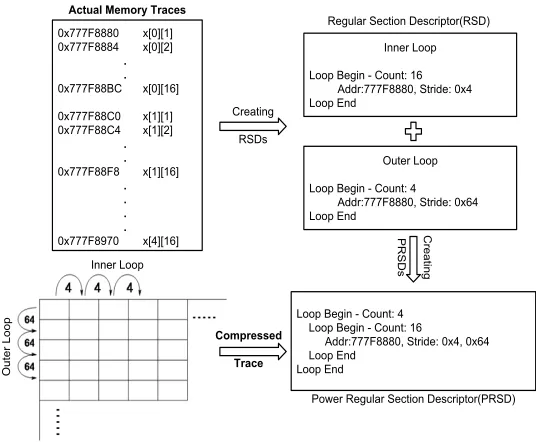
ScalaMemTrace [Bud12] is a scalable trace compression tool that is capable of collecting memory traces from uniprocessors. It uses binary instrumentation [Luk05] to collect memory traces and compresses large trace files into near constant sized trace files on-the-fly. Unlike other compression-based tech-niques that often neglect the loss of information about access patterns while removing redundant data, ScalaMemTrace (SMT) enables lossless compression for regular memory access patterns that is achieved by using special data structures like Regular Section Descriptors (RSDs) and Power Regular Section Descriptors (PRSDs). A RSD maintains details like address accessed, address stride and address type (fetch/store). A PRSD stores information such as loop count and number of RSDs within a loop.
2.2. SCALAMEMANALYSIS CHAPTER 2. BACKGROUND WORK 0x777F8880 x[0][1] 0x777F8884 x[0][2] . . 0x777F88BC x[0][16] 0x777F88C0 x[1][1] 0x777F88C4 x[1][2] . . 0x777F88F8 x[1][16] . . . . 0x777F8970 x[4][16] Creating RSDs Inner Loop Loop Begin - Count: 16
Addr:777F8880, Stride: 0x4 Loop End
Outer Loop Loop Begin - Count: 4
Addr:777F8880, Stride: 0x64 Loop End
Loop Begin - Count: 4 Loop Begin - Count: 16
Addr:777F8880, Stride: 0x4, 0x64 Loop End
Loop End Inner Loop
Outer Loop
Actual Memory Traces
Regular Section Descriptor(RSD)
Power Regular Section Descriptor(PRSD)
Creating
PRSDs
Compressed Trace
Figure 2.1 Trace Compression for nested loop using ScalaMemTrace
patterns. The replay tool [Mes07] can uncompress the traces to produce accurate memory reference counts along with the addresses as present in the original trace file.
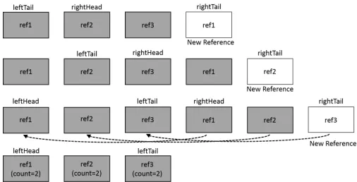
A binary instrumentation tool, Pin [Luk05], generates a raw trace file containing memory accesses, which are fed into SMT for compression. SMT recognizes the repetitive pattern [Bud12] of memory accesses and produces a compressed trace file. A stack walk is used to compute a unique signature per memory access. Since a single instruction can result in multiple memory operations, the signature acts as a criteria for the identification of memory access patterns. Figure 2.2 depicts the dynamic matching and compression of access patterns in detail. Memory references Ref1, Ref2 and Ref3 are present in the list and a new reference of Ref1 is added. This becomes the “right tail” and a matching reference is searched, which becomes the “left tail”. A reverse traversal [Bud12] of the right and left tail analyzes the matching pattern. The right and left portions are then merged, incrementing the RSD count. This process is repeated with every new reference addition.
2.2
ScalaMemAnalysis
2.2. SCALAMEMANALYSIS CHAPTER 2. BACKGROUND WORK
Figure 2.2 Dynamic Pattern Matching for Compressing Memory References.
to simulation. SMA [BM14] also provides a loopwise analysis of cache performance in an application, which helps in identifying the data structures that degrade performance. These two features give SMA a distinctive advantage compared to other tools that operate on compressed traces [Jan07; Joh01]. The following subsections provide a brief insight into SMA, which is necessary to understand the redesign for SMA-ML extension.
2.2.1 Assumptions
There are three kinds of cache misses: compulsory, capacity and conflict [Wika]. SMA [BM14] determines only capacity and conflict misses. Compulsory misses are not identified separately because they are folded into capacity misses. In SMA, the termarraycorresponds to a strided RSD in a loop. The stride multiplied with the length of a loop indicates the size of the array for dense and sequential accesses. SMA does not consider arrays partially present in the cache as it increases the code complexity prohibitively. Such arrays are assumed to benotpresent in the cache.
SMA accepts cache size, cache block size and cache associativity as configuration parameters. SMA uses a Least Recently Used (LRU) cache replacement policy, which can be easily modified to another policy by adapting the data used to populate the context information. The context information defines the size of the arrays present in the cache with respect to the size of the entire cache.
2.2.2 ScalaMemAnalysis Design 2.2.2.1 PRSD Tree Structure
2.2. SCALAMEMANALYSIS CHAPTER 2. BACKGROUND WORK
PRSD may contain RSDs as well as other PRSDs to account for nested loops.
2.2.2.2 Context-based Reuse Distance
The loop heads (PRSDs) along with loop count and number of RSDs contain context information. The context information is a measure of the number of arrays present in the cache within a specific loop. This information is maintained at each loop head and determines whether all accesses fit within the cache. This helps in deriving the cache statistics. Each loop head maintains a left context of cache capacity that contains the first set of arrays and a right context that contains the last set of arrays within a loop bounded by a cache. The cache replacement policy of SMA [BM14] can be modified by changing the ordering within the right context. In this work, the right context is ordered from Least Recently Used (LRU) to Most Recently Used (MRU).
2.2.2.3 Context Composition
The tree is initialized with a root that represents a loop head with one iteration. SMA [BM14] sequentially reads the PRSDs in the compressed trace file. As the trace is scanned, if the trace is a PRSD (loop head), then a new node is created and added as a child to the current loop head. If this trace is a RSD (memory access), then it is added as a child node to the current loop head. A child here represents a PRSD, which differs from a child node that refers to a RSD.
On discovery of a new RSD (memory access), the array is compared to the right context of the current loop head to determine if the array has been assessed previously and if it exists in the context. If so, then the array is moved to the MRU position, otherwise, if there are no conflicting arrays in right context and cache capacity permits, the array is added to the context. Cache classifiers are then assigned to arrays indicating their performance.
Loop composition occurs when all leaf nodes (RSDs) for the current loop have been added. Composi-tion is a phase where SMA identifies any conflicting arrays between the left and right contexts. Loop composition starts with a comparison between the contexts at current loop head and the array’s conflicts under a cache replacement policy to indicate conflict misses for the current loop. At the end of loop composition, the left and right contexts arerepopulated to indicate arrays accessed and present in cache. The next stage analyzes the next higher loop to determine the effect of the parent’s loop context on the cache.
2.2. SCALAMEMANALYSIS CHAPTER 2. BACKGROUND WORK
the right context, it is promoted to the MRU position. In these cases, the cache performance counters are updated to reflect the changes. When an array is already present, hits are incremented; in conflicting cases, misses are incremented. If a parent’s loop context is uninitialized, the current context data is passed to the parent because the current loop is the first access for the parent loop, and the counters remain unchanged.
CHAPTER
3
SCALAMEMANALYSIS-MULTILEVEL
REDESIGN
3.1
Design
Today’s supercomputers, clusters and commodity computers exploit multi-level cache structure to improve performance. SMA aims at assisting the user in identifying the data structures that degrade cache performance. Figure 3.1 depicts the analysis of the previous framework along with the multi-level redesign. In order to determine cache statistics, SMA analyzes the compressed traces generated by SMT. SMA builds a PRSD tree by processing the compressed file sequentially. After addition of all the RSDs for a specific loop, the tree undergoes a composition stage. As described in the previous section, the composition stage modifies, duplicates, rearranges and deletes arrays from the left as well as right contexts along multiple loop levels. This results in disintegration of RSDs and disables replay capabilities for memory access patterns. In effect, SMA only computes cache performance but does not preserve the memory miss patterns, which prevents next-level cache analysis.
3.1. DESIGN CHAPTER 3. SCALAMEMANALYSIS-MULTILEVEL REDESIGN PRSD 1 PRSD 2 . . PRSD N SMA (L1) PRSD 1 PRSD 2 . . PRSD M - Number of Hits - Number of Misses SMA -ML (L2) PRSD 1 PRSD 2 . . PRSD M - Number of Hits - Number of Misses The same SMA is instantiated
with different cache parameters depending on the cache level.
SMT 0x8..130 0x8..134 0x8..138 0x8..13c Raw Trace File Compressed Trace File (L1)
Compressed Trace File (L2)
Compressed Trace File (L3)
ScalaMemAnalysis Multi-level Redesign
Cache Parameters
(L1, L2, ...)
Cache Level: L1 Cache Level: L2 Cache Level: Ln
Figure 3.1 Workflow Through ScalaMemTrace (SMT), ScalaMemAnalysis (SMA) along with ScalaMemAnalysis-MultiLevel (SMA-ML) redesign.
each time the PRSD tree undergoes addition or composition. The LCT has miss counters associated with miss patterns depending on the miss type. These counters are updated when a miss is recorded. The basic structure of the LCT remains intact enabling perseverance of memory access patterns and generation of new miss patterns. The miss patterns computed along with miss statistics produce compressed trace files, which can be processed by SMA with next-level cache parameters. This enables multi-level cache analysis.
3.1.1 Assumptions
3.1. DESIGN CHAPTER 3. SCALAMEMANALYSIS-MULTILEVEL REDESIGN
formula:
newStride = (oldStride*loopLength)/missCount
TheloopLength is the length of the PRSD causing the miss.
3.1.2 Local Cache Tree Structure
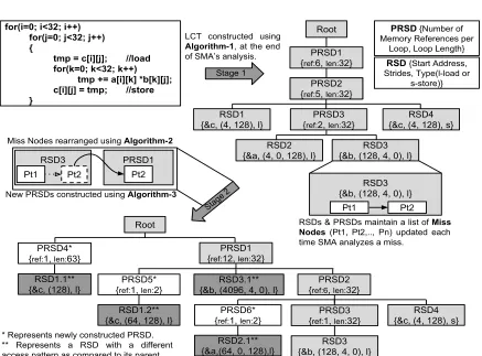
The LCT is constructed in a manner similar to that of the PRSD tree. The PRSDs act as loop heads and RSDs represent memory accesses. The structure of a sample LCT in Figure 3.2. Each PRSD denotes a loop and a certain number of memory accesses (RSDs) below it. Nested PRSDs depict nested loops. The LCT constructed using a matrix-multiplication example in Figure 3.2 consists of an outer loop (PRSD1), followed by the next-level loop (PRSD2) with two RSDs and the innermost loop (PRSD3). The innermost loop has two memory accesses, RSD2 and RSD3. The distinctive feature of PRSDs and RSDs within the LCT is that they maintain access patterns for misses, which are stored as a linked-list of Miss Nodes. A new link is added to the list each time a new miss is analyzed by SMA. Stage 1 in Figure 3.2 refers to the complete update of the LCT usingAlgorithm 1. The LCT without miss nodes, in this example, denotes the memory references to be analyzed for the L1 level cache. The PRSDs consist of:
• Loop Count: Denotes the number of loop iterations.
• Loop Size: Denotes the number of memory accesses within a loop. This establishes nested loops.
• A linked list containing details of accesses pattern for misses. Each node within the list maintains:
– The order of the accesses.
– The memory access stride pattern.
– Miss statistics along with miss stride patterns per RSD.
– The updates to miss statistics.
– Identical RSDs may exist at different levels under the same PRSD. A unique ID is used to identify them as well as maintain their location. It also helps in restructuring the file and maintaining the access patterns between loops.
3.1. DESIGN CHAPTER 3. SCALAMEMANALYSIS-MULTILEVEL REDESIGN
for(i=0; i<32; i++) for(j=0; j<32; j++) {
tmp = c[i][j]; //load for(k=0; k<32; k++)
tmp += a[i][k] *b[k][j]; c[i][j] = tmp; //store }
PRSD {Number of Memory References per
Loop, Loop Length}
RSD {Start Address, Strides, Type(l-load or
s-store)}
PRSD1 {ref:6, len:32}
PRSD2 {ref:6, len:32}
PRSD3 {ref:2, len:32}
RSD4 {&c, (4, 128), s} RSD3
{&b, (128, 4, 0), l} RSD2
{&a, (4, 0, 128), l} Root PRSD2 {ref:5, len:32} RSD1
{&c, (4, 128), l}
PRSD1 {ref:12, len:32}
PRSD3 {ref:1, len:32}
RSD4 {&c, (4, 128), s} RSD3
{&b, (128, 4, 0), l} RSD2.1**
{&a,(64, 0, 128),l} Root
PRSD2 {ref:6, len:32} PRSD4*
{ref:1, len:63} RSD1.1** {&c, (128), l}
PRSD5* {ref:1, len:2}
RSD1.2** {&c, (64, 128), l}
PRSD6* {ref:1, len:2}
RSD3.1** {&b, (4096, 4, 0), l}
RSD3 {&b, (128, 4, 0), l}
Pt1
RSDs & PRSDs maintain a list of Miss Nodes (Pt1, Pt2,.., Pn) updated each time SMA analyzes a miss.
RSD3 Pt2
PRSD1 Pt2 Pt1
Miss Nodes rearranged using Algorithm-2
LCT constructed using Algorithm-1, at the end of SMA’s analysis.
* Represents newly constructed PRSD. ** Represents a RSD with a different access pattern as compared to its parent.
New PRSDs constructed using Algorithm-3
Stage 1
Stage 2 Pt2
3.2. IMPLEMENTATION CHAPTER 3. SCALAMEMANALYSIS-MULTILEVEL REDESIGN
The above mentioned list of miss nodes is also present in RSDs along with memory access details like start address and type. Formally, an LCT is defined as a graphGwith the set of nodesP(parents),R
(leaves),M(miss nodes) andE (edges).
LCT:G= (P∪R∪M,E, ro)
wherero∈Prepresents the root andErepresents the set of edges connecting PRSD nodesPwith each other and with RSD nodesR. Furthermore, edgesEalso connect miss nodesMwith each other. An LCT nodenbuilds on the notion of a striding pattern. Forp∈Pandr∈Rwe defined
n={p,r:s≤0|p∈P,r∈R}
wheresis the stride derived from the input of the compressed trace. If the stride is greater than zero, the node is a leaf RSD; otherwise, it is a PRSD.
3.2
Implementation
3.2.1 Local Cache Tree’s Miss Pattern Updation Algorithm
The LCT’s miss statistics are updated during SMA’s addition [BM14] and composition stages. During these stages, SMA’s performance counters per loop level are constantly modified. In order to keep track of the miss patterns, each time a new miss is analyzed for a specific RSD, its unique ID is passed to the LCT asnodeID and itsmodeis updated to eitherAddorCompose. SMA’s array classifiers aid in categorizing misses into conflict and capacity misses. SMA-ML usesmissType to differentiate between the two categories. The LCT determines the miss statistics to be updated usingnodeID andmissType. The miss count and loop level is stored innewCountandlevelBit, respectively. Depending on the composition stage,levelBit may range between the next-outer and the outermost loop level. The miss count, previous stride and loop length of the PRSD causing the miss are used to calculatenewStride. The miss statistics maintain the number of miss nodes using themissNumcounter.
The LCT’s update method is described in Algorithm 1. Since the LCT updates operate on SMA information, pure conflicts, partial conflicts, varying loop levels and varying strides may need to be recalculated. A description of the composition stage is provided in Section IV.B4. At the end of populating the context information for a specific RSD, the left and the right contexts are compared and conflicting arrays are updated as conflict misses for this RSD. These updates of the LCT are depicted in lines 11-17, where for a specificnodeID,missType andAdd mode a new miss node is created in the miss statistics.
3.2. IMPLEMENTATION CHAPTER 3. SCALAMEMANALYSIS-MULTILEVEL REDESIGN
Algorithm 1Analyze Misses per RSD
1: Input:mode, newstride, updateInfo, levelBit, newCount and missType
2: Access miss statistics of (type==missType) 3: if(updateIn f o==update)then
4: for(i=0 tomissNum)do
5: if(missU sagegreater thanbitLevel)then 6: missStride=newStride
7: missU sage=levelBit
8: end if
9: end for
10: else
11: if(mode==AddANDnewCount!= 0)then 12: Create new entry
13: newCount=missCount 14: missStride=newStride 15: missU sage=levelBit 16: missNum++
17: end if
18: if(mode==Compose)then 19: for(i= 0 tomissNum)do
20: if(missU sagegreater thanbitLevel)then
21: Delete miss entry
22: missNum
-23: end if
24: if(newCount!= 0)then
25: Create new entry
26: end if
27: end for
28: end if
29: end if
level oflevelBit. This is shown in lines 18-28. If the parent’s loop is uninitialized the miss statistics of the child are passed on to the parent and the LCT is updated inupdate mode. This effectively recalculates
themissStrideandmissUsageof specific misses in the child. This is shown in lines 2-10. ThemissUsage
counter denotes the loop level at which the miss pattern was last used/updated. This eliminates any redundancy of misses during the recursive composition phase of SMA [BM14].
3.2. IMPLEMENTATION CHAPTER 3. SCALAMEMANALYSIS-MULTILEVEL REDESIGN
current/adjacent loop, it is assigned CONF_MISS and later if it conflicts with arrays in an upper loop’s context, the classifier is modified to ALWAYS_MISS for that loop’s context. During the completion of the composition stage, these array classifiers determine whether the number of misses in the current loop repeat, i.e., have to be multiplied with its parent’s loop length or not. If the misses are CONF_MISS, they are restricted to the current level and do not repeat (no multiplication). A similar pattern is followed with FIRST_MISS and CAP_MISS, where the current loop’s miss count is multiplied with the parent’s loop length for the later.
3.2.2 Miss Pattern Reconstruction Algorithm
During the addition and composition stages, the LCT’s update algorithm recordsstartAddress, missCount
andmissStrideper loop level for every miss node within a RSD. If a RSD contains more than one miss
node (miss pattern), each miss node is treated as a new (separate) RSD. The new RSD has the same start address, stack signature and type as that of the parent RSD. The loop length and stride pattern of the RSD is determined by themissCount andmissStride, respectively. The miss pattern is usually “uneven”, i.e., it does not iterate for every loop level. The uneven nature of misses is due to the cache state, which results in a non-regular pattern of capacity and conflict misses between loop levels. This unevenness is identified using themissStridearray that maintains stride information corresponding to the loop levels. This requires a rearrangement of the new RSDs to accurately maintain the miss pattern.
The reconstruction algorithm consists of two stages, (1) rearrangement of new RSDs and (2) creation of new PRSDs. These stages do not differentiate between capacity and conflict misses. (1) The rearrange-ment stage starts from the bottom-most RSD in the LCT and traverses upwards. Algorithm 2 applies to every miss node within a RSD. After all the miss nodes within a RSD have been rearranged, control moves to the next-upper RSD. This continues until the execution reaches the root. As depicted by lines 1-17 of Algorithm 2, each miss pattern identifies the uppermost iterating loop level. After determining the loop level, the miss node is added at this level and is removed from the current RSD as shown in lines 18-20. This is also shown in Figure 3.2 as a part of stage 2.
On completion of the rearrangement stage, the final phase of stage 2, i.e., creation of new PRSDs and RSDs, takes place. This stage of the algorithm iterates from top to bottom. RSDs without miss nodes are removed from the LCT. Every miss node within an PRSD and RSD is subject to steps in lines 1-8 of Algorithm 3. Each miss node identifies the lowermost iterating loop and creates a PRSD withloopLength
3.2. IMPLEMENTATION CHAPTER 3. SCALAMEMANALYSIS-MULTILEVEL REDESIGN
Algorithm 2For every Miss Node per RSD
1: fori=(maxStrideCount) to 0do 2: if(missStride[i]!=−1)then
3: Break
4: end if
5: end for
6: for j=(i) to 0do
7: if(missStride[i]==−1)then
8: Break
9: else
10: newLevel=maxStrideCount-i
11: end if
12: end for
13: fori= 0 tonewLeveldo 14: tmpNode=currentRSD 15: tmpNode=tmpNode→parent
16: end for
17: if(tmpNode→loopLevel!=currentRSD→loopLevel)then 18: CreatetmpMissPatternin tmpNode
19: tmpMissPattern=currentMissPattern
20: tmpMissPattern→tmpLevel=maxStrideCount-newLevel 21: DeletecurrentMissPattern
22: end if
algorithm, where RSD1 disintegrates into two new access patterns, RSD1.1 and RSD1.2, under PRSD4 and PRSD5, respectively. Furthermore, RSD3.1 is moved up two levels and iterates with PRSD1. The final LCT does not maintain miss information for capacity and conflict misses separately. This is because the misses at this level will be analyzed by SMA as a new set of memory access patterns. At the end of this stage, the LCT denotes the misses from L1 that are analyzed at the L2 cache level. This pattern can be used by SMA along with the next-level (L2 in this case) cache parameters to predict the cache behavior.
The final output might contain multiple individual loops that either have a single striding pattern or do not iterate with the outer encompassing loops. This occurs either due to new miss patterns formed during the composition stages of SMA or due to existence of multiple individual loops in the input trace itself. In such cases, to accurately represent the miss patterns, the single striding patterns are moved out of the outer loop, or on certain occasions the outer loop is skipped entirely. The latter is implemented in cases where all loops within a trace have unique (pairwise different) striding patterns. Since these patterns are removed from the original loop, the striding pattern is altered. In order to restore the pattern, the RSDs are sorted based on their address and previous loop level.
3.2. IMPLEMENTATION CHAPTER 3. SCALAMEMANALYSIS-MULTILEVEL REDESIGN
Algorithm 3For every PRSD and RSD in LCT
1: level=tmpMissPattern→tmpLevel 2: for(i= 0 tolevel)do
3: if(missStride[i]!=−1)then
4: Create new PRSD
5: loopLength=missCount 6: loopSize++
7: end if
8: end for
9: for j=(i) to 0do
10: if(missStride[i]!=−1)then
11: Create new PRSD
12: Create new RSD
13: loopLength=loopLengthof corresponding lower loop 14: Increment all previous loopSizes till parent PRSD
15: end if
16: end for
have the same parent RSD or parent loop level, they should be sorted in descending order of loop count for more accurate representation of miss patterns. This is valid for all the RSDs within the LCT and not restricted to single striding RSDs.
3.2.3 Regularization
SMA’s evaluation of cache performance counters is based on the cache miss equations [Gho97], which help in predicting the performance between nested loop levels as well. The left and right context information in SMA tracks misses per loop level. In case of nested loops, SMA predicts misses accurately between loops that are nested with each other, but it does not identify the patterns individually for each access or RSD. This results in new RSDs with higher aggregate miss count. When this RSD is converted into output for the next-level cache, it results in an approximate representation of the miss pattern. This has a significant effect on cases with multiple loops that have a high loop counts.
CHAPTER
4
EXPERIMENTATION
We used an AMD Opteron 6128 platform. We performed experiments to compare the execution time and accuracy of SMA-ML with a trace-driven simulator, Dinero[DI12]. The experiments consisted of matrix multiplication [Wikb] (blocked as well as unblocked), a SPEC [Hen06] benchmark suite and a NAS [Bai91] benchmark suite. All programs were compiled using gcc with O3 optimization level. In order to extract memory traces, Pin [Luk05] was used to instrument load and store instructions. From a Pin-instrumented execution of a binary, we generate (1) a compressed trace file using ScalaMemTrace [Bud12] and (2) an uncompressed trace file. The compressed trace file was fed into ScalaMemAnalysis-MultiLevel and the uncompressed trace file was fed to Dinero. Using this setup, we compared the cache performance predictions by SMA-ML with Dinero for L2 caches.
4.1
Analysis Cost
4.1. ANALYSIS COST CHAPTER 4. EXPERIMENTATION
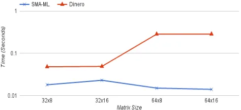
Figure 4.1 Execution Time Results for Unblocked Matrix Multiplication
Figure 4.2 Execution Time Results for Blocked Matrix Multiplication
Dinero results.
In Figure 4.1 and 4.2, the x-axis represents quadratically increasing matrix sizes and the y-axis represents time (in seconds) on a logarithmic scale. As observed in Figure 4.1, SMA-ML’s execution time remains constant whereas the execution time for Dinero increases linearly with the matrix size. This is because Dinero maintains the entire cache state by processing uncompressed traces one reference at a time so that I/O becomes a bottleneck. SMA-ML reduces the cost by analyzing the references together for each loop. This is done only once irrespective of the loop count and loop nesting levels. Furthermore, it is evident that the implementation of the LCT does not increase the analysis cost. In Figure 4.2, SMA shows up to over an order of magnitude difference in execution times compared to Dinero.
4.1. ANALYSIS COST CHAPTER 4. EXPERIMENTATION
Figure 4.3 Execution Time Results for SPEC Benchmark Suite
4.2. ACCURACY CHAPTER 4. EXPERIMENTATION
loops can break their regularity and produce less compressed trace files. The irregularity in traces can be removed by filtering the traces for those infrequent references that otherwise partition large break huge loop nestings into multiple individual loops. The SPEC benchmark Soplex and NAS benchmark Ep have such irregularity. To address this issue, we filtered out the irregular accesses from the trace, keeping the loop structure and behavior intact. After filtering, significant improvements are achieved in analysis cost and losses in accuracy are minimal. It should be noted here that filtering might not be possible when irregular memory references dominate within an application.
Figure 4.3 and Figure 4.4 depict results of the SPEC and NAS benchmark suite, respectively. The x-axis represents test cases and the y-axis depicts time logarithmically. In most cases, SMA-ML incurs less analysis cost than Dinero’s simulation cost except for SPEC Sphinx3. Sphinx3 consists of excessive number of individual access streams that produce a significant number of uncompressed trace events. As mentioned earlier, the analysis cost rises with the increase in the level of uncompressed references. In this case, that occurs due to the larger number of loops to be analyzed and the small number of references contained within each loop. These traces, when passed through SMA for the L1 level cache analysis, result in further uncompression of loops, which increases the L2 analysis cost. We will see in the next sub-section that this does not affect the accuracy of SMA-ML.
4.2
Accuracy
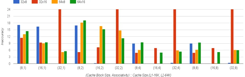
In this section, we compare the percentage miss rate of SMA-ML with Dinero to determine the perfor-mance of SMA’s redesign. In further discussion the percentage miss rate difference between SMA-ML and Dinero will be referred as accuracy. These experiments utilize data caches with 16KB and 64KB sizes for L1 and L2, respectively, with varying block size and associativity. The first set of benchmarks are matrix multiplication, unblocked as well as blocked. Figure 4.5 and 4.6 show results for unblocked and blocked matrix multiplication, respectively. The x-axis shows a large number of combinations of cache block sizes and associativities. The y-axis presents theoffset in accuracy of SMA-ML compared to Dinero. The difference in accuracy is usually below 20% but spikes up to 23% for unblocked matrix multiplication on four occasions as seen in Figure 4.5. An important metric to understand this is the L1 cache miss fraction, i.e., the number of misses passed on to L2 with respect to the total references in the trace. All four cases have L1 miss fractions below 1%, which provides insufficient data for SMA to produce accurate results, thus generating pessimistic results.
4.2. ACCURACY CHAPTER 4. EXPERIMENTATION
Figure 4.5 L2 Cache Analysis: Accuracy Results for Unblocked Matrix Multiplication
Figure 4.6 L2 Cache Analysis: Accuracy Results for Blocked Matrix Multiplication
previous cache-level does not mean that SMA-ML will always produce pessimistic results. The results shown in these two experiments consist of cases with miss fractions ranging from 0.4% to 80%, yet SMA-ML is quite accurate for most of them. During experimentation, it was observed that miss fractions below2%, i.e., very infrequent miss patterns, cause SMA to treat them conservatively as capacity misses on few occasions. Meanwhile, Dinero uses accurate simulation to determine the cache behavior. Hence, miss fractions below 2% explain SMA-ML’s pessimistic performance for regular access patterns. Note that an increase in irregularity of memory references may in turn increase the threshold for less accurate SMA-ML results to a miss fraction of 6%.
4.2. ACCURACY CHAPTER 4. EXPERIMENTATION
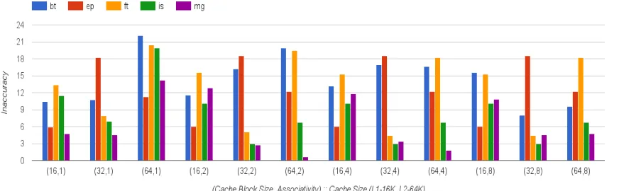
Figure 4.7 L2 Cache Analysis: Accuracy Results for SPEC Benchmark Suite
4.2. ACCURACY CHAPTER 4. EXPERIMENTATION
respectively. The x-axis displays a large combination of cache configurations testing a variety of test cases from the benchmark suites. The miss fraction of the SPEC CPU 2006 benchmarks varies between 1% to 70%, yet the inaccuracy of SMA-ML is within 20% for all test cases.
CHAPTER
5
CONCLUSION
Experiments indicate that the SMA-ML redesign does not incur additional analysis cost over the execution of SMA. The hypothesis stands valid as the analysis time remains constant irrespective of loop trip counts and provides sufficiently accurate miss rate predictions for regular access patterns compared to conventional trace-based cache simulation. Furthermore, SMA-ML maintains cache performance counters per loop level, which helps in identifying the root cause for performance degradation.
CHAPTER
6
FUTURE WORK
BIBLIOGRAPHY
[Bai91] Bailey, D. H. et al. “The NAS parallel benchmarks”.International Journal of High Performance
Computing Applications 5.3 (1991), pp. 63–73.
[BM14] Balasubramanian, N. & Mueller, F. “ScalaMemAnalysis: Compositional Approach to Multi-level Cache Analysis of Compressed Memory Traces” (2014).
[Bud12] Budanur, S. et al. “Memory trace compression and replay for SPMD systems using Extended PRSDs”.The Computer Journal 55.2 (2012), pp. 206–217.
[Wika] “Cache Miss”.URL: http://en.wikipedia.org/wiki/CPU-cache/Cache-miss(2014).
[DI12] Dinero IV, T.-D. U. C. “Simulator”.URL: http://www.cs.wisc.edu/markhill/DineroIV(2012).
[Gho97] Ghosh, S. et al. “Cache Miss Equations: An Analytical Representation of Cache Misses”. ICS ’97 (1997), pp. 317–324.
[Haq09] Haque, M. S. et al. “SuSeSim: a fast simulation strategy to find optimal L1 cache configuration for embedded systems”. Proceedings of the 7th IEEE/ACM international conference on
Hardware/software codesign and system synthesis. ACM. 2009, pp. 295–304.
[Haq11] Haque, M. S. et al. “CIPARSim: Cache intersection property assisted rapid single-pass FIFO cache simulation technique”.Proceedings of the International Conference on Computer-Aided
Design. IEEE Press. 2011, pp. 126–133.
[Haq15] Haque, M. S. et al. “Accelerating Non-volatile/Hybrid Processor Cache Design Space Ex-ploration for Application Specific Embedded Systems”. Design Automation Conference
(ASP-DAC), 2015 20th Asia and South Pacific. IEEE. 2015, pp. 435–440.
[HK91] Havlak, P. & Kennedy, K. “An Implementation of Interprocedural Bounded Regular Section Analysis”.IEEE Trans. Parallel Distrib. Syst.2.3 (1991), pp. 350–360.
[Hen06] Henning, J. L. “SPEC CPU2006 Benchmark Descriptions”.SIGARCH Comput. Archit. News
34.4 (2006), pp. 1–17.
[Jan07] Janapsatya, A. et al. “Instruction Trace Compression for Rapid Instruction Cache Simulation”. DATE ’07 (2007), pp. 803–808.
[Joh01] Johnson, E. et al. “Lossless trace compression”. Computers, IEEE Transactions on 50.2 (2001), pp. 158–173.
[JH94] Johnson, E. E. & Ha, J. “Lossless address trace compression for reducing file size and access time”.International Phoenix Conference on Computers and Communications, IEEE Press,
BIBLIOGRAPHY BIBLIOGRAPHY
[Li04] Li, X. et al. “Design space exploration of caches using compressed traces”.Proceedings of
the 18th annual international conference on Supercomputing. ACM. 2004, pp. 116–125.
[Luk05] Luk, C.-K. et al. “Pin: building customized program analysis tools with dynamic instrumenta-tion”.ACM Sigplan Notices40.6 (2005), pp. 190–200.
[Wikb] “Matrix Multiplication”.URL: http://en.wikipedia.org/wiki/Matrix-multiplication(2014).
[Mes07] Mesnier, M. P. et al. “TRACE: Parallel Trace Replay with Approximate Causal Events.”FAST. Ed. by Arpaci-Dusseau, A. C. & Arpaci-Dusseau, R. H. USENIX, 2007, pp. 153–167.
[Tau] “Tuning and Analysis Utilities (TAU)”.URL: http://www.cs.uoregon.edu/research/tau/home.php
APPENDIX
A
RSDS AND PRSDS
RSDs and PRSDs use the same format. Loopcount represents the length of the loop. Loopsize represents the number of RSDs and PRSDs within this loop. Sign represents the unique stackwalk signature. Start-value represents the start address of the memory access. Stride contains the memory access strides. Type represents the type (load/store) of the memory access. Since SMT is not restricted to uniprocessors, it maintains thread and node information as well. Tid-start-value stores the thread ID of the first thread. Tid-length represents the number of threads within a specific pattern. Tid-stride represents the distance between two thread IDs. Tid-addr-stride caters for the difference in the start-address per RSD within a thread. Similar information is stored to represent node details as well.
loopsize:6 loopcount:4 sign:0xc0ffeefeedc0ffee// gap: 0 start-value: (nil)
length: 4
stride: (nil)
tid-start-value: (nil)
tid-length: 1
APPENDIX A. RSDS AND PRSDS
tid-addr-stride: (nil)
node-id-start-value: (nil) node-id-length: 1
node-id-stride: (nil)
node-id-bit-pattern: 0x1 Sign-len = 1
Sign:0xc0ffeefeedc0ffee
APPENDIX
B
MEMORY LATENCY PREDICTIONS
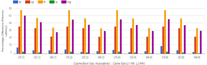
In this section, we discuss the memory latencies predicted by SMA-ML. We compare the percentage difference in L2 Memory latencies between SMA-ML and Dinero for L1 and L2 data caches of 16KB and 64KB data, respectively. The formula we use for latency calculation is as follows:
Latency = (L1_Hits * L1_Hit_Penalty) + (L2_Hits * L2_Hit_Penalty) + (L2_Misses * L2_Miss_-Penalty)
where the penalties for the cache levels are:
L1_Hit_Penalty = 1 L2_Hit_Penalty = 12 L2_Miss_Penalty = 50
APPENDIX B. MEMORY LATENCY PREDICTIONS
Figure B.1 L2 Cache Analysis: Memory Latency Results for SPEC Benchmark Suite
Figure B.2 L2 Cache Analysis: Memory Latency Results for NAS Benchmark Suite
APPENDIX
C
ADDITIONAL ACCURACY RESULTS
APPENDIX C. ADDITIONAL ACCURACY RESULTS