THE EFFECT OF INBREEDING ON THE VARIATION DUE TO RECESSIVE GENES

(1)

THE E F F E C T O F INBREEDING ON THE VARIATION

DUE TO RECESSIVE GENES

*

ALAN ROBERTSON

-4trirrtaE Breediny and Genetics Research Organization, Edirrburgh, Scotlartd Received June 25, 1951

N his classical treatment of inbreeding, WRIGHT ( 1921 ) developed the con-

I

cept of the inbreeding. coefficient F, which he defined as the correlation between the genetic constitution of the gametes in the uniting egg and sperni. This is d.irectly related to the heterozygosity remaining. in the population which is equal to l - F times the heterozygosity at the start of inbreeding. If a number of inbredelines are made without selection from a raildoni breeding population, the genetic variance due to genes which act additively increases between' lines as 2 F and decreases within lines as 1

-

F. (If inbreeding is rapid, the value 1

-

F for the genetic variance within lines is not adequate, the correct expression being 1

+

F

-

2F, where

F

is the inbreeding coefficient of the hypothetical progeny produced by randoni mating within lines in the present generation and 2 F is correct for the variance between lines.) For genes which do not act additively, there is not the same correspondence lie- tween heterozygosity and variance and the above relationships do not hold.

A s

we know little about the dominance relationships of the genes controlling continuous variation, it seemed desirable to investigate theoretically the effect of inbreeding on the variation due to genes which are conipletely recessive and to genes which show overdominance. Particular attention is given to the case in which the recessive (or quasi-recessive) is at low frequency as this is the most probable situation in natural populations.

We shall deal first with continued full-sib mating in which the results can be worked out by simple, if rather laborious, arithmetic and where the process can be most easily visualised. The more general situation of slow inbreeding in lines of' constant breeding size requires more sophisticated niatheniatics and the details of the derivations are given in an appendix. The two methods are in good agreement.

CONTINUED FULL-SIB MATING

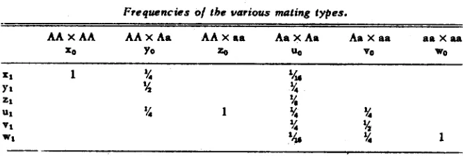
This system of mating can be treated most siniply by the inethod of mating types, originally used by JENNINGS (1916) and, subsequently with the help of matrix theory by HALDANE (1937) and ,by FISHER (1949). If only two alleles, A and a, are present in the population at a locus, there are six possible types of matings. The relative frequencies of matings of different types in any generation can be calculated from the frequencies in the previous generation

*Part of the cost of the accompanying mathematical formulae has been paid by the GALTON and MENDEL MEMORIAL FUND.

(2)

190 -4L.4N ROBERTSON

on the assuniption that the offspring are mated at random. For instance, iliatirigs Aa x aa will give offspring

5

Aa,

5

aa and if these are mated at random, one quarter of the niatings will be of the type Aa x Aa, one half Aa x

aa and one quarter aa x aa. The equations giving the frequencies of the six types in terms of the frequencies in the preceding generation are shown schematically in table 1 in which yo, for instance, signifies the frequency of

AA x Aa matings in the zero generation.

uo

+

$5

vu. If a is completely recessive to A and the phenotypic value of AA, Aa is taken

as zero atid of aa as unity, the genetic variance within the progeny of A a x .\a and !\a x aa niatings is 3/16 and 1/4 respectively, the other niatiiig types having no variation within their progeny. (Throughout the paper, " genetic variance " will be used iii the sense of all variance due to gene segregation.) The average variance within lines (each line being in this case a single mating) is 3/16 U t 1/4 v. The genetic variance between lines is easily calculated, as the expected value for the progeny is zero for all types except those repre- sented by U, v, atid w for which it is

f i ,

5

and 1 respectively.

Reading horizontally, we have, for instance, u 1 = yo

+

zo

+

TABLE 1

Frequencies

01

the various mating types.

M x A A A A x Aa A A x a a A a x A a A a x a a a a x m

=a Yo z, U0 V O wo

.I 1

v,

'4a

Yl

Y

%

21

Y

U1

v,

1

v,

%

v1

v,

Y

'Rl '& 1: 1

In the computations, we take as so, yu, zu, etc. the values for a random-bred population and evaluate the set xl, yl, zl, etc., and so on. Figure 1 shows the frequencies of mating types other than AA x AA for the case when q. = 0.1. The immediate effect of the inbreeding is to cause y to decrease and U and v

to increase. After about 6 generations, the frequencies of all types of iiiatings except AA x AA and aa x aa become practically constant relative to one an- other and then decline to zero when inbreeding is complete. At that point,

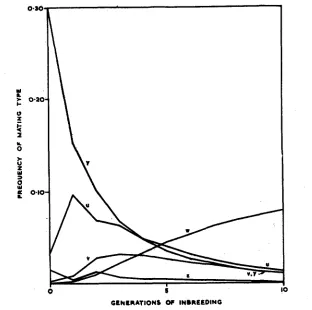
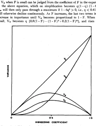
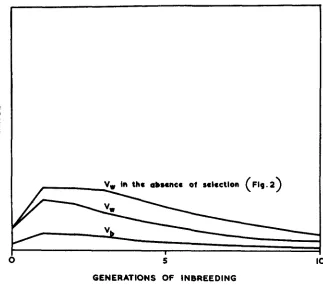
s = 0.90 and w = 0.10, as all lines become honicfzygous for either A or a. The variance within lines increases considerably in the first generittion ( F = 0.25) to 2.99 times its randoni breeding value, remains fairly stationary for two further generations, and then declines. The variance between lines increases continually as the inbreeding progresses, the rise being almost linear for the first six generations (fig. 2). Consideration of the first generation only shows that the variance within lines will only increase above its random breeding value if the frequency, q, of the recessive gene is below 0.47. At low gene frequencies, at the start almost all the a genes will be carried in matings A A x

(3)

lNBREEDING AND VARIATION 191

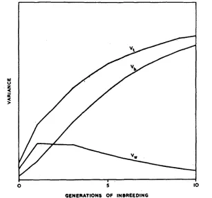
all the matings, except those of type AA x AA, will derive froin an initial entry of yo as 4q. I t follows that the shape of the curves showing the effect of inbreeding on variation will become independent of q as q decreases, as all entries will be multiples of q. Computation shows that in this case, the variance within matings reaches its maximum value of 0.207q after three generations of inbreeding (F = 0.50). Under random mating conditions, matings of type Aa x Aa will make the major contribution to the variance within mat-

I

GENERATIONS OF INBREEDING

I

FIGURE 1.-Frequencies of various mating types (except AA-x AA) with continued full-sib mating. The mating types are designated as : y (AA x Aa), r. ( A A x aa), U (Aa x Aa), v ( A a x a a ) , and w (aaxaa).

ings with freque.ncy 4q2( 1

-

q)* +- 4q2 and variance 3/16, giving an average variance of

%

qz. At its maximum, the variance within matings is therefore

0.75qa q

for the different variances when q is very low, which are not very different

from those in figure 2 for q = 0.10.

The total genetic variance rises continuously as the inbreeding progresses. When complete homozygosis is reaehed, the total variance is q ( 1

-

q); q lines having phenotypic value unity and 1 - q having value. zero. With random mating, when a fraction q2 have genotype aa and phenotype value one and

(4)

1 92 ALAN ROBERTSON

the rest have value zero, the total variance is qz( 1

-

qz)

.

Of this, the additively genetic component, the portion usually detected in genetic analyses such as heritability studies, is only Zq3( 1 - 9). When inbreeding is complete, the total variance is equal to l/q( 1 - q) times its random breeding value and 1/2 q2

times the part of the variation that can usually be detected in the absence of inbreeding. For genes which act strictly additively, the total variance at com-

W

0

T

a

*: >

~

;

FIGURE 2.-Total variance (Vt), variance within lines (Vw), and variance between lines (V,) with continued full-sih mating and q. = 0.1.

plete hoinozygosis is twice the total variance under randoni breeding conditions, the latter being, of course, equal to the additive component.

JNBREEDING I N LINES O F CONSTANT BREEDING SIZE

(5)

INBREEDING .4ND VARIATION 193

random breeding population, if there has been no selection. When inbreeding is complete, the gene frequency in each line is either 0 o r 1. The variance within and between lines can then be related to the distribution of the gene frequency in the several lines. Within a line in which the gene frequency is

'11, the genetic variance is qI2 ( 1

-

q12) 90 that the average value of the genetic

variance within lines is p2

-

p r , where the p's are the moments of the q distribution about zero. By a similar argument, the genetic variance ,between lines

w

U

z

4

>

1

a

1

I

GENERATIONS O f INBREEDING

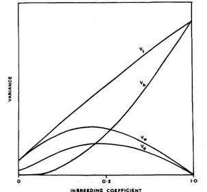
FIGURE 3.-Total variance (Vt), variance within lines (V"), and variance between lines (vb) with continued full-sib mating and q. very small.

is the variance of q12, l y

-

~ 2 . a n d the total genetic variance is ~ 1 2

-m2.

The evaluation of general expressions for the moments, and therefore of the variances, as inbreeding progresses, depends on matrix theory and is given in an appendix. The within line vdriance is given by

V,

= a ( 1 - F)

+

b( 1

-

F)*

+

c ( 1 - F)6 where a = 0.8 q( 1

-

q )

b =

-

q ( 1 - q) (1

-

2q)

(6)

1% A L 4 N ROBERTSON

When F=O, V , = a + b + c = q 2 ( 1 - q 2 ) and when F = l , V,=O. The change of V, when F is small can he judged from the coefficient of F in the expansion of the above equation, which on simplification becomes q ( 1

-

q ) (1

-

6q2). V, will then only pass through a maximum if 1

-

6q2

>

0, i.e., q

<

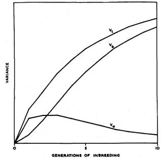
0.41 and will otherwise decline continuously. As F increases, the last two terms in V,

decrease in importance until V, becomes proportional to 1 -- F. When q is small, V, becomes q [ 0 . 8 ( 1 - F ) - ( l - F ) s + 0 . 2 ( 1 - F ) " ] , and rises to a

FIGURE 4.-Additive variance within lines (V.), total variance (V,), variance within lines (V,) and variance between lines (VI,) with random mating in a population of con- stant size with q. very small.

inaxinium of 0.280q, when F70.46, compared to q 2 ( l -q2) in the random

times the random-

0.280

lired population. The niaximum value is then roughly

-

4

breeding value, in good agreement with the value of

'z6

obtained from

continual full-sib mating.

The additive component of the variance within lines, the component de- tectable by such techniques as parent-offspring regression, is for a given line

(7)

1 N B R E E I ) l N G A N D VARI.4TION 195

2qI3 ( 1 - ql) so that the average value of this, V,, is 2 ( p a - p 4 ) . In the above

terminology this is given by .75a( 1

-

F)

+

b( 1

-

F)3

+

2c ( 1

-

F)*.

It is not possible to give simple formulae for the between line or total variance except when q is small. Then, expanding Vb as a power of F, the term with the lowest power of y is 3F3q. The total variance is then Fq. Fig- ures

4

and

5

show the behaviour of

Vt,

Vb, and V, when q is very small and when q=O.lO. The curves show clearly the main features of the effect of

inhreeding on the variance. V, and V, increase to a maximum when F = 0.4

0 0: 5

INBREEDING COEFFICIENT

1.0

FIGURE 5.-Additive variance within lines (V.), total variance (Vt), variance within lines (V,) and variance between tines (V,) with random mating in a population of con-

stant size with qn=O.l.

to 0.5 and then decline, For small values of q, V. increases as

F2

when F is low. As F approaches unity,*V, becomes equal to three-fourths of V,.

V,,

increases slowly at the start as FS but increases more rapidly when F is greater than 0.50. Vt increases almost linearly with F in both cases.

(8)

1% ALAN ROBERTSON

tilization is explicitly excluded, as of course in a bisexual organism, it is possible to have variation between lines (or rather between families) without the animals being inbred. However, the two systems are otherwise in good agreement.

GENES SHOWING OVERDOMINANCE

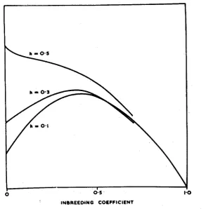
It is possible that, at some loci, the phenotypic value of the heterozygote may lie outside the range of those of the homozygotes. Of the extent and kind of such ’’ overdominance ” we know very little. As a model, it will be assumed

I

FIGURE 6.-Variance within lines for a locus with overdominance. Phenotypic values are A A = h , Aa=O, a a = 1 arid q.=O.l.

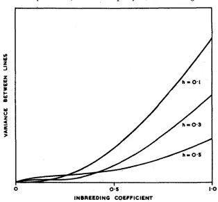
that the phenotypic values are A A = 11, :\a = 0 and aa = 1. IJsing the moment terminology, the variance hetween lines is then given by

V,=2h2pl+ ( I -211-5h2)w+4h ( l + h ) p a - (1+h)2w.

(9)

INBREEDING AND VAKlATIOK 1 Y i

arrived at for conipletely recessive genes will also apply to genes showing overdominance provided h is less than 0.2.

THE EFFECTS OF SELECTION

In the earlier analysis it was assumed that there was no selection against the recessive gene. As, in general, recessives cause some decline in fitness when they are homozygous, it seemed worthwhile to calculate the changes in variance in the extreme case when the selection against the homozygous recessive is coniplete. Here, the nieaii frequency of the recessive gene in the

FIGURE 7.-Variance between lines for a locus with overdominance. Phenotypic values are A A = h, Aa=O, aa= 1 and q.=O.l.

population of lines will not reiliain the sanie but will gradually decline as selection proceeds. The genetic variance will not depend on the inbreeding coefficient alone but also on the amount of selection and therefore on the nun1l)er of

generations that the inbreeding and selection has proceeded. There will thus be no general solution in terms of F and each inbreeding system will have to be treated separately. For continued full-sib matings, when selection against aa aniiiials is on an individual basis, there are only three possible types of

mating as shown in table 2.

The average variance within lines is 3u/l$ and that between lines is

(10)

1 98 :lLhN ROBERTSON

TABLE 2

Frequcncics o/ tbe various mating types with complete selection against the recessive /actor.

A A X A A .o

AA X Aa A a X A a

Yo U0

1 8

2

.I 1 14

Y I

?4

U1 '/4 Y

the curve for V, from figure 2 is included for coniyarison. Bbth V,, and V, rise at first and then decline to zero as inbreeding approaches coiiipletioii and all lines become A A in constitution. In the early stages, the effect of selection on the behaviour of the variance within lines is fairly small.

V,

rises to 2.69 times its random-breeding value in the ,first generation and does not decline lbelow the random-breeding value for

7

generations. With no selection, the maximum V, is 2 . 9 times the random-breeding value and it takes 10 generations to decline to that value again. The selection against the recessive on this model is the most stringent possible on an individual basis and one can safely make the generalization that in the early generations of full-sib

5

IO

(11)

INBREEDING AND VARIATION 1 9

mating, selection will not greatly affect tlie behaviour of the variance within lines. If the inbreeding proceeds more slowly, selection will be more iniyortant as it will have more opportunity to take effect.

T H E PERFORMANCE OF THE: LINES I N CROSSING

From the practical point of view iiiore interest attaches to the yerforniance of the crosses between lines than to that of the lines theniselves. The performance of the crosses made between members of a group of lines is often discussed in terms of ‘’ general combining ability ” and

‘‘

special combining

ability.” The ” general combining dbility ” of a line refers to the average per-

formance of the crosses between that line and all the other lines. The ’’ special combining ability ” of a particular cross refers to the difference between the

performance of the cross and what would have been expected from the geii- era1 combining abilities of the parent lines. In mathematical terms, the performance of a particular cross Pij between the ith and jtl’ lines is given by

Pij = ni +ai

+

aj

+

ail

where in is the mean of all crosses, ai, aj are the general combining abilities of the ith and jth lines and aij is the interaction term, the special combining ability. The term ‘‘ top-cross ” refers to the crosses made between a line and

a sample of individuals from the random-bred population. The average top- crossing performance of a line should be equal to the general combining ability in crosses with lines drawn without selection from the random-bred population, because the gametes froin a group of inbred lines made without selection are exactly equivalent to a random sample of gametes from the randoni-bred population. In a similar manner, a series of crosses made at random between completely inbred lines made without selection are equivalent to a group of individuals drawn from the random-bred population.

Consider two lines in which the gene frequencies of the recessive are q1,

‘12. Then, assuming complete dominance, the average performance of the cross

(12)

200 .lL.-lN ROBERTSON

pect, it is the best cross between nieiiibers of a group of lines that is important. For a given nuniber of lines, the probable superiority of the best cross above the mean will be proportional to the standard deviation between crosses and will be proportional to the first power of F if q is small.

The correlation between the performance of lines in crossing when the lines are partially inbred with the performance when inbreeding is complete

is of some practical interest. . \ s inlreeding causes the gene frequencies to deviate Ixtween lilies but does not change the average gene frequency in the

In

W

In

U)

:

V

z

W

I

t

W

0

W

0 z

4 >

5

a

0 . 5 1-0

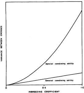
FIGURE 9.-Relative contribution of general and specific conibining ability to the vari- ance bet\\een crosses with change in inbreeding. q = 0.1.

whole population of lines, it follows that the expected gene frequency in coin-

(13)

INBREEDING ANI) VARIATION 20 1

future performance of a cross between two lines on its present performance will always be unity, irrespective of the stage at which the lines are measured.

From this, it follows that the correlation between future performance and present performance will he equal to

variance of present performance

v-

variance of future perfarmance

In particular, for general combining aldity, this equals

and for the performance of a specific line cross it is

q'( 1 -9) F(F

+

2q -Fq)

F(F

+2q

-Fq)

c = c

\vhich is equal to 1; when q is small.

'Hie correlation hetween the phenotypic value of a line and its general cnnrhining ability will he generally for a single gene fairly close to one, being

:L correlation hetween q1 and qI2.

VARIATION D U E TO M A N Y RECESSIVE GENES

We have been dealing above with the variation due to a single recessive gene. I n practice, the genetic variation may he expected to be due to many genes with different gene frequencies and effects of different magnitude. Fortunately, this does not greatly complicate the pictiire and many of the results c?ii he taken over directly from the single gene case. The resultant w-iance will be merely the sun1 of the variance due to the separate genes, so that a generalization can be made a b u t the variation due to recessive genes at frequencies less than about 0.3, that the within line variance will increase until F is in the region of 0.5 and then decline and that the between line variance wid1 increase at first as

F3.

Indeed, the presence of variation due to many genes means that as far as the within line variance is concerned, lines \vi11 deviate less from the predicted hehaviour than they would if the variation were due only to a single gene. In B similar way, the formulae referring

to the crossing performance of lines for genes of low frequency can also he

taken over to the general case as can those for the correlations and regression of future performance and present performance of crosses.

DISCUSSION

(14)

202 .%LAY ROBERTSON

1948). Apart from the possibilities arising from the present paper, there are three other possible causes for such a phenomenon.

( a ) Natural selection for heterozygotes may he opposing the trend towards homozygosis produced by inbreeding.

(b) In many characters, the greater part of the variation is environniental in origin and therefore will not be affected by inbreeding. In characters like egg production index in poultry or litter size in swine, 'the changes in genetic variance may be undetectable against the hackground of the environmental variance.

( c ) The inbred lines may differ from the random-'bred stock in their re- sponse to environmental changes. WRIGHT (1935) has described a line of guinea-pigs in which a proportion of animals are otocephalic. There is con- siderable variation in head shape within the line which, on testing, was found to be not genetic in origin. It seeins that the line has shifted towards some critical threshold in the process of head formation over which a proportion of

the environmental variations takes the animals in the course of development, resulting in a variety of different ahnornialities of head shape.

To these three factors affecting the total variation within lines, we may now add a fourth-that the variation due to recessive genes at low frequency will increase with inbreeding until F is about 0.50 and may not return to its original value until F reaches close to 1.

W e are still fairly ignorant about the exact behaviour of the genes respon- sible for continuous variation. In some characters, e.g., fat percentage in milk in cattle, it is likely that the genes are acting mostly in an additive manner. In other, in particular, characters with low heritability that show inbreeding depression, e.g., egg production index in poultry, yield in maize, a high pro-

portion of the genetic variation might he due to recessive or overdominant genes. Such genes will generally he held at a lcnv frequency in the population I)! natural selection. The possihle increase of the genetic variance due to such genes with increasing inhreeding has therefore some practical importance. 'There are some writers who maintain that animals whose performance is in- ferior are so hecause they are homozygous for deleterious recessives. They argue that the only way to improve the general level of the stock is to uncover the recessives by inhreeding and so to produce a population with a uniformly high level of performance. In fact, even with stringent selection against such recessives. it will take several generations of hrother-sister matings in which the recessives are segregating out before the genetic variance within such an inbred population will decline to its original value. This is only one of several objections to such a pror, * a nime.

The results presented here may be of some use in providing a possible explanation for some peculiar experimental results but it is douhtful whether they can he of any precise value in the analysis of continuous variation. When the variation is due to several recessive genes at different frequencies, this treatment can only supply a general description of the probable behaviour

(15)

INBREEDING AKD VARI.\TIOS 20.3

The only situation in which the gene frequencies are known accurately-in

a cross between two inbred lines-the position is complicated by linkage.

J n discussing the variation due to several genes almve, it has been assume!l that in the initial random-bred popidation there is no correlation between the genes present at adjacent loci in a gamete. I n the F2 of a cross I)etween

two inbred lines, there will he such a correlation Iletween genes at adjacent loci and any analysis will tell 11s almout the properties of such blocks of genes rather than of the individual genes. In the absence of overdominance at indi-

vidual loci, such blocks of genes will tend to show overdominance themselves,

due to the usual covering-up of recessives. It seems therefore that unfortunately the use of such a cross cannot tell 11s much about the dominance relationships of the individual genes.

SUhIMARY

The effect of inbreeding on the variation due to recessive genes has been treated theoretically both for the case of continued full-sib mating and in line5

of small breeding size. If the recessives are at low frequency, the variation within lines increases to a maximum when F is close to 0.50, and declines to zero when inbreeding is complete. The additive coinponent of the variance within lines behaves in a similar manner. The variance between lines is small at first, increasing as F3 when F is small. The total variance in the population

of lines increases almost linearly with F. The variance in the performance of crosses between lines is made up of a component due to the general conibiniiig aldity of lines proportional to F and to a component ascribable to the special combining ability in particular crosses proportional to F?. The special coni-

hining ability thus becomes much more important as inbreeding progresses. The effects of overdominance and selection are also briefly treated.

LITERATURE CITED

FISHER, R. A., 1949 The Theory of Inbreeding. viii t 120 pp. Edinburgh. Oliver and

Boyd.

HAI.DANE, J. B. S, 1937 Some theoretical results of continued brother-sister mating. J. Genet. 34: 265-274.

J R N N I N G S , H. S., 1916 The numerical results of diverse systems of mating. Genetics 1: 53-89.

PEASE, M. S., 1948 Inbreeding in poultry livestock improvement. Proc. 8th World's

Poultry Congress, 3.M.5. WRIGHT, S., 1921

WRIGHT,

s.,

and 0. N. EATON, 1923 Factors which determine octocephaly in guinea-pigs.

Systems of mating. Genetics 6: 111-178.

J. Agr. Res. 26: 161-181.

APPENDIX

A GENERAL DERIVATION OF THE RELATIONSHIP OF THE GENETIC VARIANCE To THE

COEFFICIENT OF INBREEDING, F

(16)

201 ALAN ROBERTSON

groups being distributer1 hinoniially with mean nq and index n. The next generation is then the repetition of this process, each line giving rise to a group of lines whose gene frequencies are binomially distributed about the mean of the parent line. If the number of lines is constant, the sample of existing lines can be considered as a random saniple from the above hypothetical population.

Consider, in the rt" generation, the lines (having frequency f , ) in which the gene frequency is q,. These lines will then by the ahove operation give a new group of lines in which the moments about zero of the gene frequencies are by the usual formulae for a binomial distribution,

The moments of the total population of lines will be the sum of the moments of the groups of lines, arising from each value of ql with appropriate weights fi.

1

n

= - r Pi +

(I

-

Pa (the r subscripts referring to generations.)

Similarly we have three other equations relating the moments in the (r t 1)" generation to those in the r" generation, which can be written diagrammatically as follows:

r P * r P a rFs r k

r+l P1 1

1 3

r + l P r na

-

n -(I

-

;)

(I

-

;)

(I

-

;)

Thus, knowing the values in the zero generation, we could work out the values in any generation. By the use of matrix theory, it is possible to 0btain.a general expression for the moments in any generation. For a four-rank matrix such as the above, there are

four latent roots, XO, XI, XZ, b, and to each latent root there corresponds a latent vector t ( a linear function of the moments) such that :

r +:te

ho

r b

r + a t l = L r t r

r + I t a = ha rta

(17)

INBREEDING AND VARI.\TION 205

Knowing the zero value for the latent vectors, t, we can easily calculate the values in the rth generation as .to = “to io‘ and so on, and therefore also calculate the moments by expressing then1 as functions of the t’s. As the elements to the right-hand of the diagorlal are zero, tlie four latent roots are simply the entries in the main diagonal. As an example nf tlie evaluation of the latent vectors, consider tlie vector tr corresponding to the rnnt A:.

We may express t2 as alpl

+

a+?

+

alpl t a+pr. We then ohtain the roeficieiits by cquatiw the coefficients of the fi’s deriving from the t recurrence equations with those deriving

from the P reciirrence equations. Writing 1

- -

= b. etc. we have

a4Al = a4hi

a& = a4

-

+

aihl 1

n

6ha n

7x1 311

nr n

ho

n’ na n

asha = a4-

+

a,-

+

a J l

a l l 2 = a 4

-

+

as - + a ,

-

+

alho giving

Then

a4 = 0

a, = 1 (M arbitrary value) 3

2 a l e--

1

a1 =

-

2

1 3

2 2 t a = - P i - - P a + P i

The four equations for the t’s are then:

Aa = I t o = PI

1

n

x i =

1-- t 1 = -P1+ P l

1 3

2 2

tl = -Pi

--

Pa + P i

n - 1 6 n - 7

5n-6 Sa-6

hi= (1

-

;)

(1

-

;)(I

-

;)

[,=-- P I + - Pa- 2Pi P4 If n is lorle, r e may write

1 6

5 5

t ) = - -Pi +-Pa

-

2 P i + P L ~

Correspondingly, we have four equations for the moments in terms of the latent vectors.

P S ” b

Pa = t o + t l

3

p, = to + - t l

+

t a

2

9

p4 = to + - t ,

+

2ta

+

t l

(18)

206 ALAN ROBERTSON

In the zero generation, we have o Pn = q" giving

* o = q

a t 1 = - d l

-

q)

1

0 t s =

-

- q ( l

-

q) +

q y l

-

q)l

5

Then for V w in the rth generation,

r v w = r p a

-

r P 4

1

is the expected relative decline in heterozygosis each

generation,

(1

-3

is the proportion remaining after r generations and i s equal to

l * F . If n is large, then ( l - $ r = ( l - : r r = ( l - F y . T h u d h : = ( I - F Y ap-

proximately and A: = (1

-

FF, giving

V, = a(1 - F )

+

b(1- FY

+

c ( 1 - F ) 9 Similarly,

rv-,

= 2(, p,

-

p,)

3

4

= -a(1

-

F)

+

M 1 - F)' t 2 4 1

-

F)6

vt

is given by the erpression, Vt = pa

-

pi where PI = q

-

q(1- q ) ( l - F)

= q'

+

q(l

-

q)F, giving

Vt = q(1- 9) [q( 1

+

(1)

+

F( 1

-

2q')

-

F'q( 1

-

q)l

If q is small, this reduces to Fq.

simple expression seems to exist. Expansion gives, in order of powers of F,

VI, is then obtained as Vt-V, but unfortunately no

(19)

I N B RE EI)I N G AN D V AR 1A T I ON ₂₀₇ For the genes showing overdominance, the general principles are the same except that the values for the first and third moments also enter into the calculation.

The variance between the performances of the lines on top-crossing to the original ~ml~ulatiori can easily he calciilated. If the gene frequency in a line is (11 then the proportion of honiozygons recessives in back-crossing to tlie original populatioii (in whicli the gem frequency is q ) is qql, and this \vi11 be the iiieaii pheiiotype value of tlic ww.

I hevariaiicerequiredistlienc~var q, = q ~ ( ~ ~ - p , ~ ~ ~ ~ i ~ l q - q ( l - q ) (1 -F)-$1 = F q " ( l - q ) which increases as the first power of I;. If we cross two lines in which the gene frequriicirs are q,, qs the mean phenotypic value of the cross is q3*. To calculate the total variance between such crosses, we have to find tlie variance of qlqr when q1 and q2 are independent

members of the q distribution. Actually the moments about zero of such a distributioii of

a product are the products of the moments of the parent distributions. A s in this case, the two samples are from the same distribution, the moments about zero of the product distribution are the square of the moments of the q distribution. In terms of those moments tlie variance between line crosses = pi" - pl'

-.

= q'( 1 - 9) F ( F

+

2q - Fq)