ABSTRACT
XU, MINGYANG. Probabilistic Models for Aspect-based Opinion Mining. (Under the direction of Dr. Nagiza F. Samatova.)
The Web now has an overwhelming amount of textual information available, such as online reviews, news articles, and blogs, which often contain important information, such as the popular subjects being discussed, opinions, and sentiment toward these subjects. One important problem over such large collections of unstructured text is automatically mining aspect-level opinions. Aspect-based opinion mining mainly consists of two core tasks: (1) extraction of relevant aspects and opinions, and (2) sentiment classification of the discovered aspects and opinions. For example, given a review about a cellphone, “The battery is great and durable”, “battery” should be extracted as an aspect, “great” and “durable” should be extracted as opinions, and both “great” and “durable” should be classified as positive opinions.
In recent years, various probabilistic models, especially topic models, have been proposed to tackle one or both of the above tasks. Traditional topic models primarily focus on the first task, extracting major topics that pervade a corpus. Each of the topics is represented by a set of semantically related individual words, which are the major aspects and opinions in the given corpus, and are discovered based on higher-order word co-occurrences. Extracting topics based on word co-occurrence requires a large amount of data, e.g., thousands of documents, to provide reliable statistics for generating coherent topics. In practice, when there is a limited amount of data available, these methods typically suffer.
Complementing the methods based on word co-occurrence, sentiment-topic models try to directly address both tasks of aspect-level opinion mining. Each topic discovered, and each word in the corpus, is assigned a sentiment, e.g., negative and positive. Each discovered topic contains only aspects and opinions with the same sentiment. The words in different topics can have different sentiments. Existing sentiment-topic models typically rely only on the local context of a word when determining its sentiment, ignoring more global indicators, which often results in incorrect sentiment classification.
To further tackle the second task of aspect-based opinion mining, we propose an opinion mining topic model, called LOT. Our model can simultaneously discover relevant aspects and opinions, and assign accurate sentiment to words by incorporating public word-sentiment knowledge. Experimental results for topic coherence, document sentiment classification, and a human evaluation all show that our proposed model achieves significant improvements over several state-of-the-art baselines.
© Copyright 2018 by Mingyang Xu
Probabilistic Models for Aspect-based Opinion Mining
by Mingyang Xu
A dissertation submitted to the Graduate Faculty of North Carolina State University
in partial fulfillment of the requirements for the Degree of
Doctor of Philosophy
Computer Science
Raleigh, North Carolina
2018
APPROVED BY:
Dr. R. Raju Vatsavai Dr. Steffen Heber
Dr. Dennis R. Bahler Dr. Nagiza F. Samatova
BIOGRAPHY
ACKNOWLEDGEMENTS
TABLE OF CONTENTS
LIST OF TABLES . . . vi
LIST OF FIGURES . . . vii
Chapter 1 Introduction . . . 1
1.1 Lifelong Learning Topic Model . . . 5
1.2 Opinion Mining Topic Model . . . 6
1.3 Phrase-based Topic Model . . . 6
Chapter 2 Lifelong Learning Topic Model . . . 8
2.1 Introduction . . . 8
2.2 Related work . . . 10
2.3 Knowledge mining . . . 11
2.3.1 Mining must-links and cannot-links . . . 11
2.3.2 Dealing with issues of knowledge . . . 13
2.4 LDA . . . 15
2.5 LKT . . . 17
2.6 LLT . . . 19
2.7 Experiments . . . 21
2.7.1 Datasets and experimental setting . . . 21
2.7.2 Topic coherence . . . 25
2.7.3 Human evaluation . . . 26
2.8 Conclusion . . . 29
Chapter 3 Opinion Mining Topic Model . . . 30
3.1 Introduction . . . 30
3.2 Related Work . . . 32
3.3 LDA . . . 33
3.4 ASUM . . . 36
3.5 LOT Model . . . 37
3.6 Evaluation . . . 40
3.6.1 Experimental Setup . . . 40
3.6.2 Topic Coherence . . . 42
3.6.3 Document Sentiment Classification . . . 44
3.6.4 Human Evaluation . . . 45
3.7 Conclusion . . . 51
Chapter 4 Phrase-Based Topic Model . . . 53
4.1 Introduction . . . 53
4.2 Related Work . . . 55
4.3 Bigram Topic Model . . . 57
4.4 LDA Collection Model . . . 57
4.5.1 TNG . . . 58
4.5.2 Inference in KTP . . . 61
4.6 Experiments . . . 61
4.6.1 Phrase Coherence with Different Amount of Knowledge . . . 64
4.6.2 Human Evaluation . . . 69
4.7 Conclusion . . . 70
Chapter 5 Conclusion and Future Work . . . 71
5.1 Conclusion . . . 71
5.2 Future Work . . . 72
LIST OF TABLES
Table 2.1 Notation used in this paper . . . 15 Table 2.2 List of category names: 1000E and 100E (1st row), 1000NE and 100NE
(2nd row). . . 22 Table 2.3 Example must-links and cannot-links discovered from ”Cellphone“. . . 27 Table 2.4 Example topics of LLT, LKT and AMC from the Cellphone, Sci tech,
Beauty domain. Errors are marked in red. . . 28 Table 2.5 Domains selected for human evaluation. . . 28 Table 2.6 Human evaluation results. P@5, P@10, P@15 as well as the average
percentage of coherent topics for each model. . . 28
Table 3.1 Notation used in this paper . . . 34 Table 3.2 List of category names: 1000E and 100E (1st row), 1000NE and 100NE (2nd
row), and the amazon review dataset used for training word embeddings (3rd row). . . 41 Table 3.3 Example words of the opinion list created by the authors in [24]. Left
column is positive opinion words. Right column is negative opinion words. 42 Table 3.4 Example words with sentiment scores in SentiWordNet [4]. Left column
is the opinion words. Right column is the sentiment scores, which are represented as (positivity, negativity). . . 43 Table 3.5 Example words of our pre-identified general positive and negative opinions.
These words are manually selected from the opinion word list. . . 44 Table 3.6 Accuracy of document-sentiment classification on our four datasets (with
10 topics). . . 45 Table 3.7 Example positive and negative topics of JST, ASUM and LOT from the
category of Headphones. Opinion words are shown in italics. Incorrect aspect words and opinion words are underlined. Non-specific opinion words are marked by a dashed line under them. All these errors are also marked in red. . . 47
Table 4.1 Notation used in this paper . . . 56 Table 4.2 List of category names: 1000E and 100E (1st row), 1000NE and 100NE
(2nd row). . . 62 Table 4.3 Example topics discovered by TNG and KTP. Errors are italicized and
marked in red. . . 66 Table 4.4 Examples of phrase knowledge discovered from the domain “GPS”. . . 68 Table 4.5 Examples of phrase correlation knowledge discovered from the domain
LIST OF FIGURES
Figure 1.1 Example of how traditional topic models work on online reviews. . . 2
Figure 1.2 Example of how sentiment-topic models work on online reviews. . . 3
Figure 1.3 Example of how phrase-based topic models work on online reviews. . . 4
Figure 1.4 Overview of the dissertation chapters and how they relate to the research objectives. . . 5
Figure 2.1 An example of using word embedding for mining knowledge. . . 12
Figure 2.2 An example of the topic embedding. . . 13
Figure 2.3 An example of learning topical word embedding where word “apple” only appears in topic 1 and topic 4, which are about “food”. The learned new word embedding of word ”apple“ is more relevant to “fruit”. . . 14
Figure 2.4 The graphical model of LDA. . . 16
Figure 2.5 The graphical model of LKT. . . 17
Figure 2.6 The graphical model of LDA. . . 20
Figure 2.7 Average topic coherence score on 1000ER dataset with different number of learning iterations . . . 22
Figure 2.8 Average topic coherence score on 1000NER dataset with different number of learning iterations . . . 23
Figure 2.9 Average topic coherence score on TMN dataset with different number of learning iterations . . . 23
Figure 2.10 Topic coherence score on all datasets with 5 topics. . . 23
Figure 2.11 Topic coherence score on all datasets with 15 topics. . . 24
Figure 2.12 Topic coherence score on all datasets with 45 topics. . . 24
Figure 3.1 The graphical model of LDA. . . 35
Figure 3.2 The graphical model of ASUM. . . 36
Figure 3.3 Graphical model of LOT . . . 37
Figure 3.4 Average topic coherence score on 1000E dataset with different number of topics. . . 45
Figure 3.5 Average topic coherence score on 1000NE dataset with different number of topics. . . 46
Figure 3.6 Average topic coherence score on 100E dataset with different number of topics. . . 47
Figure 3.7 Average topic coherence score on 100NE dataset with different number of topics. . . 48
Figure 3.8 Human evaluation results of aspect-word labeling for the domains from 100E and 100NE. . . 48
Figure 3.9 Human evaluation results of aspect-word labeling for the domains from 1000E and 1000NE. . . 48
Figure 3.11 Human evaluation results of opinion-word labeling for the domains from
1000E and 1000NE. . . 49
Figure 3.12 Human evaluation results of word specificity labeling for the domains from 100E and 100NE. . . 49
Figure 3.13 Human evaluation results of word specificity labeling for the domains from 1000E and 1000NE. . . 50
Figure 3.14 Human evaluation results of topic labeling for the domains from 100E and 100NE. . . 50
Figure 3.15 Human evaluation results of topic labeling for the domains from 1000E and 1000NE. . . 50
Figure 4.1 Graphical Model of BTM. . . 58
Figure 4.2 Graphical Model of LDA Collection Model. . . 59
Figure 4.3 Graphical model of the TNG model. . . 60
Figure 4.4 Average phrase coherence score of bigrams discoverd by the models from 20 categories of 1000R and 100Rdataset . . . 63
Figure 4.5 Average phrase coherence score of trigrams discoverd by the models from 20 categories of 1000R and 100Rdataset . . . 63
Figure 4.6 Average phrase coherence of bigrams over 20 categories of 100R dataset with different ratio of external knowledge incorporated. . . 64
Figure 4.7 Average phrase coherence of trigrams over 20 categories of 100R dataset with different ratio of external knowledge incorporated. . . 65
Figure 4.8 Average phrase coherence of bigrams over 20 categories of 1000Rdataset with different ratio of external knowledge incorporated. . . 65
Figure 4.9 Average phrase coherence of trigrams over 20 categories of 1000R dataset with different ratio of external knowledge incorporated. . . 65
Figure 4.10 Human evaluation results of phrase labeling of trigrams . . . 66
Figure 4.11 Human evaluation results of phrase labeling of trigrams . . . 67
Figure 4.12 Human evaluation results of topic labeling of bigrams . . . 67
CHAPTER
1
INTRODUCTION
There is now an overwhelming amount of textual information available on the web, such as online reviews of products, news, and blogs. This data contains important information, such as the major aspects (subjects) that people are discussing, and corresponding opinions and sentiments. For example, the aspects and opinions in online reviews can help customers to better understand why other customers like or dislike an item, or help inform merchants about how to improve their products. However, manually extracting this type of information requires enormous human efforts. Therefore, there is an important and growing need for techniques capable of mining aspect-level opinions from texts, which mainly consists of two core tasks: (1) extracting relevant aspects and opinions, and (2) sentiment classification of the discovered aspects and opinions. For example, given a review about a cellphone, “The battery is great and durable”, “battery” should be extracted as an aspect, “great” and “durable” should be identified as opinions, and both “great” and “durable” should be classified as positive opinions.
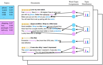
phone 0.09 watch 0.05 strap 0.04 USB 0.01 ...
shipping 0.07 box 0.04 packagin 0.03 delivery 0.02 ...
Topics Documents AssignmentsWord-Topic DistributionTopic
Figure 1.1 Example of how traditional topic models work on online reviews.
with higher probability in that topic. An example of how traditional topic models work is shown in Figure 1.1. Each of the discovered topics consists of a set of related aspects and opinions.
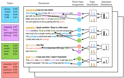
To tackle both tasks for aspect-based opinion mining, another important class of topic models has been proposed, called sentiment-topic models [17, 18, 25, 27, 30, 40, 50], which are able to simultaneously discover topics and assign sentiment to words. Figure 1.2 shows an example of how sentiment-topic models work. Different from traditional topic models, each document in this type of model is assigned a topic distribution as well as a sentiment distribution. Each discovered topic is labeled with a sentiment, and the words in a single topic should have the same sentiment. Note that the ratings of the reviews are unknown to the model.
Most of the existing topic models operate under the “bag of words” assumption, which means that word order is not considered in these models. Consequently, as topics are simply a collection of individual words, the meaning or definition of a discovered topic can be hard to understand. For example, the relevance of words “deep” and “machine” under the same topic is hard to understand. Conversely, their relevance is very clear by seeing their phrases, “deep learning” and “machine learning”.
phone 0.09 watch 0.05 strap 0.04 USB 0.01 ...
shipping 0.07 box 0.04 packagin 0.03 delivery 0.02 ...
Topics Documents AssignmentsWord-Topic DistributionSentiment
strap 0.09 watch 0.05 loose 0.04 dirty 0.01 ...
restockin 0.07 ship 0.04 excessive 0.03 expensive 0.02 ...
Topic Distribution
Figure 1.2 Example of how sentiment-topic models work on online reviews.
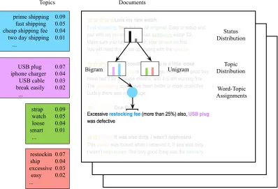
word. Longer phrases, composed of more than two words, can be formed by simply combining sequential bigrams. Half of the generated topics are represented by a set of individual words, while the other half of the topics are represented by a set of N-gram phrases.
Despite the progress in this area, there are still many challenges, summarized as follows:
1. For traditional topic models, topics are typically discovered based on word co-occurrences - if the given corpus is small and contains very limited co-occurring words, the quality of
the resulting topics may suffer.
prime shipping 0.09 fast shipping 0.05 cheap shipping fee 0.04 two day shipping 0.01 ...
USB plug 0.07 iphone charger 0.04 USB cable 0.03 break easily 0.02 ...
Topics Documents
Word-Topic Assignments
Topic Distribution Unigram
Bigram
restockin 0.07 ship 0.04 excessive 0.03 easy 0.02 ...
strap 0.09 watch 0.05 loose 0.04 smart 0.01 ...
Status Distribution
Figure 1.3 Example of how phrase-based topic models work on online reviews.
3. Phrase-based topic models, similar to traditional topic models, also require a large amount of data, e.g., thousands of documents, to provide reliable statistics for discovering meaningful phrases and coherent topics. When the amount of data is limited, which is often the case in practice, the quality of the topics and phrases discovered suffers.
In this thesis, we propose three models to address the challenges enumerated above. The rest of this thesis is summarized as follows:
• In Chapter 2, we propose a knowledge-based topic model and a lifelong learning topic model for discovering coherent topics from both small and large corpuses.
• In Chapter 3, we propose an opinion mining topic model to tackle both of the tasks for aspect-based opinion mining. Our model is able to assign accurate sentiments to words and discover coherent topics. In addition, the topics discovered by our model consist of more specific opinions.
Figure 1.4 Overview of the dissertation chapters and how they relate to the research objectives.
modeling respectively. As with our LKT and LLT models, our phrase-based topic model can discover meaningful phrases and coherent topics from both small and large corpuses.
1.1
Lifelong Learning Topic Model
Topic models have been widely used for discovering latent topics from a corpus. To generate more coherent topics, knowledge-based topic models were proposed as a way of incorporating prior knowledge about word correlation information obtained from public sources. However, this prior knowledge may actually contribute to incoherent topics, because it is general public knowledge and may contain knowledge that is irrelevant or incorrect for the specific, relatively small test dataset.
Recently, latent embedding structured topic models were also proposed to generate coherent topics by exploiting latent vector representation of words (latent embeddings). However, this type of topic model assumes that words are generated independently, losing rich and important word correlations.
To address these issues, we propose a new topic model, called the LKT model (Latent embedding structured Knowledge-based Topic model), which incorporates word correlation knowledge as well as latent embedding structure. Specifically, the word correlation knowledge incorporated in our model includes must-links (pairs of words that should be in the same topics) and cannot-links (pairs of words that should not be in the same topics). This knowledge is automatically mined using our knowledge mining method from the latent embeddings.
Lifelong learning Topic model). In each iteration of the learning process of LLT, new word correlation knowledge is mined using the topic-word distributions generated from our LKT model in the previous iteration. This new knowledge is incorporated into LKT to generate more accurate topic-word distributions, which are used for mining better knowledge in the next learning iteration. As a result, our LLT model can learn from the past to continually gain better results. Experimental results over several datasets show that our proposed topic models can generate much more coherent topics than state-of-the-art methods.
1.2
Opinion Mining Topic Model
To simultaneously discover coherent topics and assign accurate sentiments to words, we propose LOT (Latent embedding structured Opinion mining Topic model). Similar to our LKT model and LLT model, LOT is also structured using latent embeddings to discover coherent topics. However, unlike LKT and LLT, LOT is able to assign sentiment to words. Each discovered topic contains a set of semantically related words. All of the words in a given topic are assigned the same sentiment. The words in different topics can have different sentiments.
In LOT, we model specific opinion words and general opinion words separately. Both general opinions and specific opinions are used for assigning sentiment to words and documents, while only specific opinions will appear in the discovered topics. In this way, LOT can discover more specific opinions than existing sentiment-topic models.
To assign more accurate sentiment to words, in addition to the document-sentiment distri-bution that existing models rely on, we also exploit a word-sentiment distridistri-bution, which is estimated based on the sentiment of all the instances of each word in the entire corpus and the sentiment information of each word in public sentiment lexicons. The intuition behind our approach is that document-sentiment distributions can only be used to derive the sentiment of each word based on local context, whereas word-sentiment distributions provide the sentiment of each word in a general, more global, context. By simultaneously estimating and utilizing these two distributions, our model can assign more accurate sentiment to words. Experimental results for topic coherence, document sentiment classification, and human evaluation all show that our proposed model achieves significant improvements over several state-of-the-art baselines.
1.3
Phrase-based Topic Model
words, as phrases are typically more meaningful. However, these models typically require large amounts of data to provide reliable statistics for phrase-based topic modeling, thus limiting their performance in scenarios with limited data.
CHAPTER
2
LIFELONG LEARNING TOPIC MODEL
2.1
Introduction
Topic models, such as Latent Dirichlet allocation (LDA) [6], have been widely used for discovering major themes–topics–that pervade a collection of text documents. A topic refers to a set of words sharing a common sense. Traditional topic models generate topics based on higher-order word co-occurrences but can suffer when there are limited word co-occurrences in test dataset. In recent years, knowledge-based topic models [3, 13, 14, 39] were proposed to incorporate prior knowledge into topic models to generate more coherent topics. Such knowledge typically includesmust-links defined as pairs of words should be in the same topic, e.g., (apple, banana), andcannot-links defined as pairs of words should be in the different topics, e.g., (banana, red). However, existing topic models that directly incorporate knowledge in this way can suffer from a domain adaptation problem, where the general knowledge base will contain irrelevant knowledge to a more specific, smaller test dataset. For example, (apple,iphone) is a correct must-link in general; however, in the context of a specific dataset about “fruit”, applemay only mean “fruit” and not “IT company”. Thus, (apple,iphone) would be an incorrect must-link for this dataset. Therefore, solely relying on prior knowledge, such as must-links and cannot-links, may still generate incoherent topics, due to the potential low relevance of the provided knowledge.
as shown in [29, 41, 44]. Although these types of topic models can take advantage of word embeddings, they assume that words are generated independently, ignoring the important and useful knowledge of word correlations, such as must-links and cannot-links.
Therefore, rather than solely relying on prior must-links/cannot-links or the structure based on latent word embeddings, in this paper, we first propose a new topic model called the LKT model (Latent embedding structured Knowledge-based Topic model). Our LKT model is structured based on latent embeddings, but it’s also able to incorporate both must-links and cannot-links. The strength of our LKT model is that it can take advantage of both latent embedding-structured topic models and knowledge-based topic models to generate more coherent topics. Specifically, our model is structured using two types of embeddings: (1) word embeddings pre-trained on a large external corpora to capture the semantic meanings of words in general context and (2) topic embeddings learned in our model to capture the semantic meaning of latent topics. To leverage the knowledge of must-links and cannot-links, we incorporate them in the sampling procedures of our model to help learn more accurate topic embeddings. The details of LKT can be found in Section 2.5.
To solve the domain adaptation problem mentioned above, we also propose a knowledge mining method that can mine reliable knowledge (must-links and cannot-links) directly and automatically from the test dataset. Specifically, we exploit word embeddings pre-trained on a large external corpora to determine semantically related and unrelated words (must-links and cannot-links). While these embeddings provide a wealth of semantic information, they may not be entirely relevant to the relatively small (and perhaps more specific) test dataset, causing wrong knowledge to be mined. Therefore, instead of simply using this pre-trained word embedding for mining knowledge, we learn topical word embeddings for mining must-links and cannot-links, which are new embeddings that incorporate the pre-trained word embeddings as well as the topic-word distributions generated by the topic model from test dataset. With this combination, we are able to reduce irrelevant word meanings that are not present in test dataset. The detail of our knowledge mining is describe in Section 2.3.
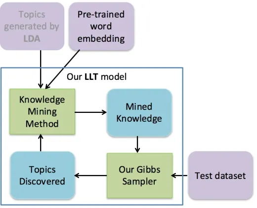
To further improve our model, we propose a lifelong learning topic model based on latent embeddings, called the LLT model (Latent embedding structured Lifelong learning Topic model) that connects our knowledge mining method and our LKT model via a lifelong learning framework. Our LLT model is based on the idea of lifelong machine learning (LML) [10, 46, 49], with the intuition being to simulate the learning process of humans; i.e., learning from the past results to improve future results. The main steps of our lifelong learning framework can be summarized as follows:
1. Pre-train a word embedding model on a large public corpora.
3. Learn topical word embeddings based on the topic-word distributions and pre-trained word embeddings.
4. Mine must-links and cannot-links using the topical word embeddings.
5. Generate new topic-word distributions by incorporating must-links and cannot-links into our LKT model. Then, repeat steps (3) to step (5).
We first mine our initial knowledge using the topic-word distributions generated by running LDA [6] on the test data, as shown in Steps (1) to (4). Then, our LKT model incorporates this mined knowledge to generate more coherent topics in Step (5). Then, as part of our
lifelong learning process, steps (3) to (5) are repeated. During each iteration over these steps, new topical word embeddings are learned using the topic-word distributions generated by our LKT model in the previous iteration, ultimately improving the mined knowledge. In turn, our LKT model incorporates the new knowledge to generate new and more accurate topic-word distributions(more coherent topics) to be used in next iteration, and so on. The intuition behind our approach is that good knowledge leads to more coherent topics and more coherent topics lead to better knowledge. Existing methods [11, 12] were also proposed to automatically and iteratively mine the knowledge for topic modeling; however, compared to our approach, these methods have several key differences, as discussed in Section 3.2.
In summary, the main contributions of our paper are:
• A knowledge-mining method, based on topical word embeddings, that is able to mine must-links and cannot-links automatically from the test dataset (Section 2.3).
• A new topic model, called LKT, structured using latent embeddings and having the capability of incorporating both of must-links and cannot-links to generate more coherent topics (Section 2.5).
• A lifelong learning topic model, called LLT, that connects our proposed knowledge mining method and our LKT model. It is able to learn from the past results to continually generate more coherent topics (Section 2.6).
2.2
Related work
topic model and our LLT model is a lifelong learning topic model that combines our proposed knowledge mining method and the LKT model under a lifelong learning framework.
With regard to our LKT model, our LKT model first differs by its ability to deal with
the domain adaptation problemof potentially mining wrong knowledge in the context of the
test dataset. For example, [56] proposed a Markov Random Field regularized LDA model by incorporating word similarity knowledge into topic modeling. [3] and [14] incorporated prior provided must-links and cannot-links to improve their topic modeling. However, all these models assume that the prior knowledge is correct without dealing with the potential of wrong knowledge. [13] dealt with wrong knowledge, though their model only incorporated must-links and did not include cannot-links. In contrast, LKT can handle both types of knowledge while also dealing with the domain adaptation problem and other types of wrong knowledge.
Furthermore, our LKT model is structured using latent embedding, which none of the existing knowledge-based topic models are. There have been some recently proposed topic models that exploit word embeddings to structure their models [15, 41, 43]. However, none of these models are able to incorporate must-links or cannot-links. Our LKT model is also structured using latent embedding while also being able to incorporate must-links and cannot-links.
With regard to our LLT model, the most related work is AMC [11] and LTM [12], which were also proposed to automatically and iteratively mine knowledge for topic modeling. However, LTM only mines must-links iteratively and AMC only mines cannot-links iteratively. In contrast, our model is able to automatically and iteratively mine both must-links and cannot-links. In addition, LTM and AMC need to mine their knowledge from additional datasets with a large number of domains and relevant content to the test dataset. However, if the content of the test dataset is unknown, then it is unlikely that one will find appropriate datasets for this process. Even the content is known, finding or building relevant datasets with a large number of domains requires a substantial human involvement. In contrast, our model is able to mine the knowledge simply from the test dataset, avoiding these complications entirely.
2.3
Knowledge mining
In this section, we present our knowledge mining method for mining must-links and cannot-links at first, and then our approach for dealing with potential wrong knowledge.
2.3.1 Mining must-links and cannot-links
Figure 2.1 An example of using word embedding for mining knowledge.
we learn topic embeddings based on the pre-trained word embeddings and the topic-word distributions generated by the topic model from the test dataset. The details of learning the topic embeddings are introduced in Section 2.5, as it’s related to our LKT model. The pre-trained word embeddings are able to provide the semantic meaning of each word in general, while the learned topic embedding of a topic is used to represent the semantic meaning of that topic.
Finally, we learn the topical word embeddingaw for wordwby concatenating its pre-trained word embedding and the corresponding weighted average topic embedding as follows:
aw =ww⊕λ¯w (2.1)
where the ⊕denotes the concatenation operation.ww denotes pre-trained word embedding for word w. λ¯w denotes the weighted average topic embedding of the topics containing word w, which is defined as follows:
¯
λw =
P
t∈T P(w|λtwT)λt
P
t∈T P(w|λtwT)
(2.2)
where T denotes the topics containing word w, λt denotes the embedding for topic t, and P(w|λtwT) denotes the probability that wordwbelongs to topict, as defined in Equation 3.6.
Figure 2.2 An example of the topic embedding.
topic model: if appleonly appeared in topics about “food”, then the meaning of learned topical word embedding for apple gets much closer to “fruit”, not “IT company name.” In addition, topical word embedding is the key to performing lifelong learning in our approach, as described in Section 2.6.
Thesemantic similarity of two words is computed as cosine similarity of their corresponding topical word embeddings. In the process of mining must-links and cannot-links, We define two fixed threshold:πm andπc. A pair of words is considered a must-link if the similarity score is aboveπm. The pair is considered a cannot-link if the similarity score is lower thanπc.
2.3.2 Dealing with issues of knowledge
There are many potential issues with the mined knowledge, some of which are also discussed in Chen and Liu [11, 14]. First of all, given two mined must-links may also imply a wrong must-link. For example, (apple, iphone) and (apple, grape) as must-links may imply wrong must-link (grape, iphone).
To solve this problem, in our LKT model, for each word in each document, we sample a must-link containing the word at first, then only must-links semantically related to the sampled must-link will be incorporated as shown in Section 2.5. Two must-links containing word ware
Figure 2.3 An example of learning topical word embedding where word “apple” only appears in topic 1 and topic 4, which are about “food”. The learned new word embedding of word ”apple“ is more relevant to “fruit”.
semantically related only if (w1, w2) also forms a must-link.
Another important issue with must-links is wrong knowledge. In order to handle wrong knowledge, we take advantage of NPMI score (Normalized Pointwise Mutual Information) [7]. It is based on word co-occurrence and is proven to be very effective to measure the association between two words as mentioned by Lau et.al [26]. NPMI score is defined as:
NPMI(w, w0) = log
P(w,w0) P(w)P(w0)
−logP(w, w0) (2.3)
where P(w) denotes the frequency of a document containing the wordw.P(w) is defined as:
P(w) = #D(w)
#D (2.4)
P(w, w0) denotes the frequency of a document containing both word wandw0 and is defined as:
P(w1, w2) =
#D(w1, w2)
#D (2.5)
(Section 2.5) when incorporating the cannot-links, because most pairs of words rarely appeared together in a single document, so a low NPMI score doesn’t necessarily lead to a correct cannot-link.
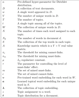
Table 2.1Notation used in this paper
α Pre-defined hyper-parameter for Dirichlet distribution.
D A collection of text documents. w A single word appeared inD. V The number of unique words inD.
T The number of topics.
t A single topic among all of the topics. W The collection of unique words inD.
N The number of times each word assigned to each topic.
Nd The number of words in documentd.
S The collection of the top words in each topic. A Knowledge matrix which is aV ×V real value
matrix.
πc The threshold for mining cannot-links. πm The threshold for mining must-links. µ L2 regularizer constant.
τ The parameter for controlling the level of must-links’ effect.
m The set of mined must-links. c The set of mined cannot-links.
w Pre-trained word embedding for each word inW.
a Learned topical word embedding for each unique word in S.
λ The collection of topic embedding. z Topic assignment to a word. θ Topic distribution for a document.
2.4
LDA
Figure 2.4 The graphical model of LDA.
graphical model is shown in Figure 3.1, whereNdis the number of words in document d. The generative process is summarized as follows:
1. For each document d, draw a topic distributionθd∼Dir(α);
2. For each topict, draw a word distribution φt∼Dir(β);
3. For each word wi in each documentd,
(a) sample a topiczi∼M ulti(θd);
(b) sample a word wi ∼M ulti(φzi);
The probability of sampling topict to wordwi in document d, is defined as:
P(zi =t|z, α, β,w) =
n−t,wii+β
PW
w0=1(n−t,wi0 +β)
n−d,ti +α
PT
t0=1(n−d,ti0+α)
(2.6)
Wherend,t denotes the number of times the words in documentdare assigned with document t, nt,w denotes the number of times the words assigned with topict.
The probability of word wi in topictis defined as:
P(wi|t, β) =
nwi,t+β
PW
w0=1(nw0,t+β)
(2.7)
λ
Figure 2.5 The graphical model of LKT.
2.5
LKT
In this section, we introduce our proposed LKT model. In our model, we exploit the framework using in GPU model [39] to incorporate must-links and M-GPU [11] to incorporate cannot-links. However, unlike GPU and M-GPU, our LKT model is structured using latent embeddings, which is very effective in topic modeling, as shown in [8, 15, 41, 43].
In our approach, a must-link means a pair of words that should be in the same topic. In contrast, a cannot-link means a pair of words that should be in different topics. Thus, in our LKT model, for incorporating must-links, the basic idea is when a word wis assigned to topic t in our Gibbs sampling procedure, we also assign a certain number of word wm to topict, given the must-link (w, wm), to increase the probability that wandwm appear in the same topic. For incorporating cannot-links, we re-sample cannot wordwc in cannot-link (w, wc) to the different topic than the topic containingw to decrease the probability that wandwc appear in the same topic.
The graphical model of LKT is shown in Fig. 2.5, where Nd denotes the number of words in document d,T denotes the number of topics,V denotes the size of the vocabulary and D denotes the input documents. Our LKT model exploits pre-trained word embeddings denoted bywand topic embeddings denoted by λtto structure our model. The generative process of our proposed LKT model is:
1. For each document d, draw a topic distributionθd∼Dir(α);
2. For each word wi in each documentd,
(a) sample a topiczi∼P(zi|θd);
(b) sample a word wi ∼P(wi|λziw T);
where P(zi|θd) and P(wi|λziw
T) are multinomial distributions. We define the probability of
word embedding win LKT as:
P(w|λtwT) =
exp(λt·ww)
P
w0∈Wexp(λt·ww0) (2.8)
The rationale being that the semantic similarity of two words is determined by the cosine similarity of the corresponding vectors. Thus, the higher the similarity between λt andww the higher the probability of the wordw appearing in topic t.
The conditional probability of topic tsampled to ith word in documentd, say w
i, is defined as:
P(zi =t|z−i, α,λ,w)
∝(Nd,t−i+α) exp(λt·wwi)
P
w0∈Wexp(λt·ww0)
(2.9)
whereNd,t−i indicates the number of times the words in document dare assigned to topictexcept the current assignment. Nguyen et.al [43] also follow this idea to define their latent component, but without incorporating any knowledge.
In LKT, we incorporate mined must-links and cannot-links for each wordwiin each document dfrom the test dataset as follows:
Incorporating must-links: We incorporate must-links in LKT via a knowledge matrix A, a V ×V real value matrix whereV is the number of unique words in the input dataset.A is initialized as an identity matrix. Then, for each pair of mined must-link (w, wm),A is defined as:
Aw,wm=τ·NPMI(w, wm)
Awm,w=Aw,wm
(2.10)
PMI is defined as equation 3.13 andτ is the parameter for controlling how much we can trust the must-link.
Given a set of must-links containing word wi assigned to topict, we sample one must-link, saysm, that is the most related to topic tusing the following conditional distribution:
P(sm = (wi, wm)|λtwT) = P(wi|λtwT)·P(wm|λtwT) (2.11)
where (wi, wm) denotes the sampled must-link and P(w|λtwT) refers to the probability of word w generated by topictbased on Equation 2.8.
distribution:
P(sc=wc|z, α)∝
Ndc,t+α
PT
t0=1(Ndc,t0+α)
(2.12)
where dc denotes the document of wordsc. Then, the cannot wordsc is re-assigned to another topic. In order to handle wrong cannot-links, for each candidate topict, except its original topic zc, we only assignscto the topic with higher probability of word wc based on equation 2.8. If there is no candidate topic with higher probability, sc is still under its original topic, else sc is re-sampled to the new topic based on the conditional distribution:
P(zsc =t|z
−sc, α,λ,w)∝(N−sc
dc,t +α)
exp(λt·wsc)
P
w0∈Wexp(λt·ww0) (2.13)
whereN−sc
dc,t is the number of times topic t assigned to the words except thesc in documentdc.
Learning topic embeddings: After incorporating the mined must-links and cannot-links, the topic embedding λtis then estimated using MAP estimation. The negative log likelihood with L2 regularization of the collection of documents for each topic Lt is defined as:
Lt=−
X
w∈W
( X
(w,wm)∈mw
Aw,wmNt,wm+Nt,w)
λt·ww−log
X
w0∈W
exp(λt·ww0)
+µkλtk22
(2.14)
where µ denotes the L2 regularizer constant,mw denotes the set of sampled must-links and related must-links containing wordw, and A is the knowledge matrix defined in Equation 2.10. Since the topic embedding is used for mining knowledge, so initial topic embedding is estimated without considering knowledge.
The MAP estimation is then applied to estimate λt by minimizingLt. The derivative with respect to thejth element of topic embedding λ
t is defined as:
∂Lt ∂λt,j
=− X
w∈W
( X
(w,wm)∈mw
Aw,wmNt,wm+Nt,w)
ww,j− X
w0∈W
ww0,j P(w0 |λtwT)+ 2µλt,j
(2.15)
2.6
LLT
In this section, we present the overall lifelong learning algorithm of our LLT model as shown in Algorithm 1.
Figure 2.6 The graphical model of LDA.
Algorithm 1 LLT(D,w, N, S) for iter= 1 to r do
λ← learnTE(N,w)
a← learnTWE(λ,S) m,c← mineKnowledge(a) N ← LKT(D, m, c)
2.7
Experiments
In this section, we demonstrate that our proposed LKT and LLT model are able to generate much more coherent topics than the following state-of-the-art topic models:
DF-LDA[3]: A knowledge-based topic model that can incorporate user-provided must-links and cannot-links.
LTM [12]: A lifelong learning topic model that can automatically and iteratively mine and incorporate only must-links.
AMC [11]: A lifelong learning topic model that can only iteratively mine and incorporate cannot-links.
LF-LDA [43]: A topic model structured using latent embedding that does not incorporate any word correlation knowledge.
I-AMC: A variation of AMC by replacing the original knowledge mining method in AMC with our proposed knowledge mining method.
AMC-Wiki: A variation of AMC by allowing AMC mine its knowledge from large wikipedia corpus.
LKT: Our proposed knowledge-based topic model structured using latent embedding, also with the capability of incorporating automatically mined must-links and cannot-links.
LLT: Our proposed lifelong learning topic model based on latent embedding that can automatically and iteratively mine and incorporate both must-links and cannot-links.
We evaluate the baseline models and our models based on two tasks:topic coherence score[39]
andhuman evaluation, which are the most common approaches for evaluating the coherence
and quality of the topics generated by a topic model [11, 12, 39, 56].
2.7.1 Datasets and experimental setting
To ensure an unbiased comparison, we directly use the datasets that were used in the papers of the basline models we compare against. Among our test datasets, 1000ER1 contains reviews from 50 types of electronic products; 1000NER1 contains reviews from 50 types of mixed non-electronic products; Each domain contains 1000 reviews. and TMN2 contains descriptions of English RSS news from 7 categories. Each category contains around 4600 news. All of the datasets are pre-processed as described in their original papers [11, 43].
The pre-trained word embedding used in LLT, LKT and LF-LDA is public to download, which is generated by training skip-gram model on Google News Dataset3 containing 100 billion
1Download at: https://www.cs.uic.edu/ zchen/ 2
Download at: https://github.com/datquocnguyen/LFTM
3
Table 2.2 List of category names: 1000E and 100E (1st row), 1000NE and 100NE (2nd row).
Alarm Clock, Amplifier, Battery, Blu-Ray Player, Cable Modem, Camcorder, Cam-era, Car Stereo, CD Player, Cell Phone, Computer, DVD Player, Fan, GPS, Graphics Card, Hard Drive, Headphone, Home Theater System, Iron, Keyboard, Kindle, Lamp, Laptop, Media Player, Memory Card, Microphone, Microwave, Monitor, Mouse, MP3Player, Network Adapter, Printer, Projector, Radar Detector, Remote Control, Rice Cooker, Scanner, Speaker, Subwoofer, Tablet, Telephone, TV, Vacuum, Video Player, Video Recorder, Voice Recorder, Watch, Webcam, Wireless Router, Xbox Android Appstore, Appliances, Arts Crafts Sewing, Automotive, Baby, Bag, Beauty, Bike, Books, Cable, Care, Clothing, Conditioner, Diaper, Dining, Dumbbell, Flash-light, Food, Gloves, Golf, Home Improvement, Industrial Scientific, Jewelry, Kindle Store, Kitchen, Knife, Luggage, Magazine Subscriptions, Mat, Mattress, Movies TV, Music, Musical Instruments, Office Products, Patio Lawn Garden, Pet Supplies, Pillow, Sandal, Scooter, Shoes, Software, Sports, Table Chair, Tent, Tire, Toys, Video Games, Vitamin Supplement, Wall Clock, Water Filter
words. In addition, words in the dataset without a corresponding pre-trained word embedding are removed.
The parameters for all of the baselines are set at the suggested values in their original papers. For LLT and LKT, the parameters are estimated on the domain Music from 1000NER. This domain is not used for evaluation in our experiments. Our parameters are set as: α = 0.1, β = 0.01 as suggested by [32],µ= 0.01, τ = 3.35, πm = 0.4, andπc= 0.05.
Figure 2.8 Average topic coherence score on 1000NER dataset with different number of learning iterations
Figure 2.9 Average topic coherence score on TMN dataset with different number of learning itera-tions
-1650 -1550 -1450 -1350
LLT LKT I-AMC LF-LDA AMC LTM DF-LDA
1000ER 1000NER TMN
T
opi
c
cohe
re
nc
e
sc
or
e
Test with 5 Topics
-1600 -1500 -1400 -1300 -1200 -1100 -1000
LLT LKT I-AMC LF-LDA AMC LTM DF-LDA
1000ER 1000NER TMN
T
opi
c
cohe
re
nc
e
sc
or
e
Test with 15 Topics
Figure 2.11Topic coherence score on all datasets with 15 topics.
-1550 -1450 -1350 -1250 -1150 -1050 -950
LLT LKT I-AMC LF-LDA AMC LTM DF-LDA
1000ER 1000NER TMN
T
opi
c
cohe
re
nc
e
sc
or
e
Test with 45 Topics
2.7.2 Topic coherence
In this section, we evaluate our proposed models and baseline models using topic coherence score [39]. Specifically, the topic coherence score is defined as:
P(t, V(t)) = M
X
m=2 m−1
X
l=1
logD(v (t)
m, v(t)l ) + 1 D(vl(t))
(2.16)
where V(t) is a list of theM most probable words in topic t. A smoothing count of 1 is included to avoid taking the logarithm of zero. D(v, v0) denotes the number of documents containing both word v andv0,D(v) denotes the number of documents containing word v. A higher score
indicates that the generated topics are more coherent.
As our proposed LLT model is able to learn from the past results to generate more coherent topics, we first evaluate our models and baseline models over multiple learning iterations. Fig. 2.7, Fig. 2.8 and Fig. 2.9, show the average topic coherence score (over each domain) on all datasets in each learning iteration. For this experiment, we had each model generate 15 topics, as this was the setting used in papers of baseline models. All models were tested on each domain of each dataset and we let AMC and LTM mine the knowledge from the remaining domains of that dataset. However, LLT only mines knowledge from the individual domain being tested. Even so, the results in Fig. 2.7, Fig. 2.8 and Fig. 2.9 show that LLT outperforms the baseline models significantly (p < 0.001 based on student paired t-test) in each learning iteration. Moreover, LLT has a better learning ability with much more improvement between each learning iteration, compared to AMC and LTM. Since LKT cannot mine knowledge by itself, we feed the knowledge mined by LLT in first learning iteration to LKT in all of our evaluations. As LKT and LF-LDA don’t have a learning ability, their performance doesn’t change with different learning iteration. However, LKT still outperforms baseline models significantly (p <0.001 based on student paired t-test).
In addition, assess the performance of AMC (as AMC outperforms LTM across all datasets) using large unlabeled data, like our model. Since the raw data of Google News dataset is not available, we use another very large wikipedia dataset for AMC mining knowledge. Specifically, we divide the large wikipedia dataset 4 into 50 smaller datasets randomly. Then, AMC mines knowledge from this divided wikipedia dataset, denoted as AMC-Wiki. The results show that the performance of AMC-Wiki is even slightly worse than AMC on some datasets, which mines knowledge from the rest of the labeled domains in the dataset. A possible reason is that 50 smaller datasets creates enough number of “domains”, as required by AMC. However, the content of each domain is very different, and the AMC model needs the content of each domain
to be relevant to the test dataset and each other.
Finally, we evaluate the performance of all models on all datasets while varying the number of topics, as shown in Fig. 2.10, Fig. 2.11 and Fig. 2.12. The learning iteration is set as 4 for LLT and LTM, because the topic coherence of all models typically stabilize after 4 learning iterations (see Fig. 2.7, Fig. 2.8 and Fig. 2.9). It’s set as 3 for AMC as suggested in its original paper. For DF-LDA, we feed the knowledge mined by our model, because DF-LDA can’t mine knowledge by itself. The results illustrate that LLT and LKT outperform all baseline models significantly (p <0.001 based on student paired t-test), regardless of the number of topics generated.
Effectiveness of our knowledge mining method and our LKT model: In above evaluations, LKT incorporates the knowledge mined by our knowledge mining method. In order to evaluate the effectiveness of our knowledge mining method and LKT model individually, we replace the knowledge mining method of AMC with our proposed knowledge mining method, denoted as I-AMC in Fig. 2.10, Fig. 2.11 and Fig. 2.12. The results indicate that I-AMC achieves a much better performance than AMC, demonstrating the effectiveness of our knowledge mining method. However, our LKT still outperforms I-AMC significantly demonstrating the effectiveness of our LKT model.
2.7.3 Human evaluation
In this experiment, we test whether the generated topics are coherent from the perspective of humans. In general, we follow the steps and setting of the human evaluation conducted in [11, 12, 56], except we recruit more human judges in our evaluation. Specifically, each topic model generates 15 topics and each topic keeps 15 top words. We compare our LLT and LKT model with AMC and LTM in this evaluation, which achieved a higher topic coherence score when generating 15 topics in topic coherence. We recruited five human judges who are familiar with amazon products and reviews for this evaluation. We selected six domains from tested datasets, as shown in Table 2.5, based on how well all of human judges are familiar with the domain, because if human judges have no background knowledge of a domain, they can’t make accurate evaluations. As is common for evaluating topic models [11, 12, 39], our human evaluation consisted of two tasks: topic labeling and word labeling.
Topic labeling: The human judges are asked to mark each topic generated by each model as coherent or incoherent. If most of the words in the topic share the same “sense”, the topic is marked as coherent topic; otherwise, the topic is marked as incoherent.
Word labeling: Only the topics marked as coherent in topic labeling are used for word labeling. Human judges are asked to mark each word in each topic as coherent if the word is related to the topic or incoherent if the work is not related to the topic.
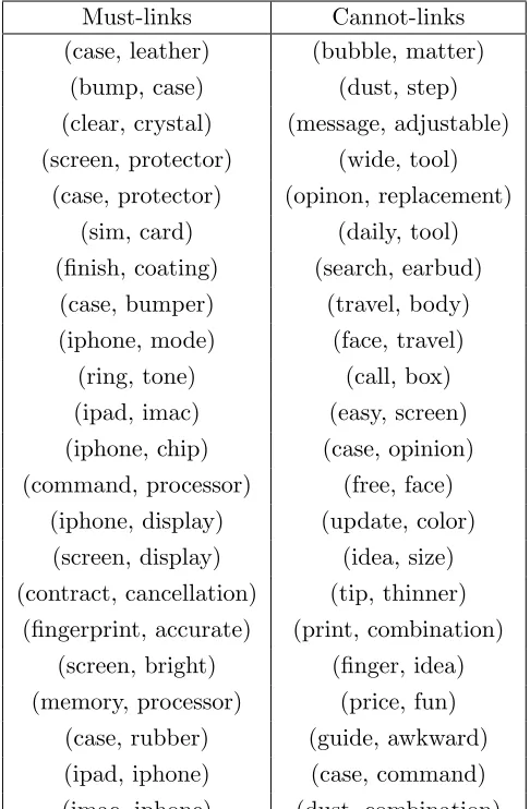
Table 2.3 Example must-links and cannot-links discovered from ”Cellphone“.
Must-links Cannot-links
(case, leather) (bubble, matter)
(bump, case) (dust, step)
(clear, crystal) (message, adjustable) (screen, protector) (wide, tool)
(case, protector) (opinon, replacement) (sim, card) (daily, tool) (finish, coating) (search, earbud)
(case, bumper) (travel, body) (iphone, mode) (face, travel)
(ring, tone) (call, box)
(ipad, imac) (easy, screen) (iphone, chip) (case, opinion) (command, processor) (free, face)
(iphone, display) (update, color) (screen, display) (idea, size) (contract, cancellation) (tip, thinner)
(fingerprint, accurate) (print, combination) (screen, bright) (finger, idea) (memory, processor) (price, fun)
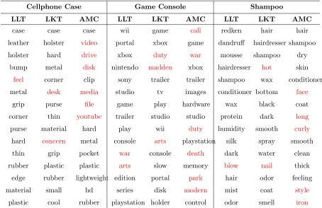
Table 2.4 Example topics of LLT, LKT and AMC from the Cellphone, Sci tech, Beauty domain. Errors are marked in red.
Cellphone Case Game Console Shampoo
LLT LKT AMC LLT LKT AMC LLT LKT AMC
case case case wii game call redken hair hair
leather holster video portal xbox game dandruff hairdresser shampoo
holster hard drive xbox duty war mousse shampoo dry
bump metal disk nintendo madden xbox hairdresser hot skin
feel corner clip sony trailer trailer shampoo wax conditioner
metal desk media studio tv images conditioner bottom face
grip purse file game play hardware wax black coat
corner thin youtube trailer studio studio protein dark long
purse material hard play wii duty humidity smooth curly
hard concern metal console arts playstation silk spray smooth
thin grip pocket war console death dark water clean
rubber plastic plastic arts slow memory blow nail thick
edge rubber lightweight edition portal park hair odor feeling
material small hd series disk modern mist coat style
plastic cool rubber playstation holder control odor smell iron
Table 2.5 Domains selected for human evaluation.
1000ER 1000NER TMN
Cellphone Sports Health
Computer Beauty Sci tech
Table 2.6 Human evaluation results.P@5,P@10,P@15 as well as the average percentage of coher-ent topics for each model.
Models P@5 P@10 P@15 Coherent topics
LLT 91.4% 90.7% 87.3% 80.4%
LKT 90.1% 86.7% 84.2% 79.9%
AMC 83.7% 78.5% 77.1% 73.2%
topics being marked as coherent. In topic models, the words in each topic are ranked based on their probability assigned to that topic. So for word labeling, the models are evaluated using P@n–the percent of the top n words that are marked as coherent, as defined in [42]. In our experiments,nis set to 5, 10 and 15.
The human evaluation results are shown in Table 2.6. The Cohen’s Kappa agreement scores for topic labeling and word labeling are 0.92 and 0.86 respectively, meaning the human judges make very similar decisions on both of topic labeling and word labeling. For topic labeling, LLT and LKT generates more than 7.2% and 6.7% coherent topics than the baseline models. For word labeling, both of LLT and LKT outperform baseline models significantly (p <0.01 based on student paired t-test) forP@5,P@10, andP@15respectively. These results demonstrate that our proposed LLT and LKT can generate more coherent topics. Table 4.3 shows some example topics generated by our proposed LLT, LKT and AMC model [11], because AMC outperforms other baseline models in most of our evaluation. The example topics are selected from all the topics in our human evaluation with the highest agreement of decisions made by human judges. The incoherent words marked by human judges in each example topic are marked in red in Table 4.3. It’s obvious that topics generated by LLT and LKT are more coherent.
2.8
Conclusion
CHAPTER
3
OPINION MINING TOPIC MODEL
3.1
Introduction
There are now numerous websites and apps that offer online reviews of products, restaurants and other items. These reviews usually contain specific opinions of users and customers towards different aspects (features) of the items being reviewed. Awareness of these opinions is critical both for merchants to improve their products and for customers to make purchasing choices. However, manually extracting these opinions requires enormous human efforts. Therefore, there is an important need to automatically mine aspect-level specific opinions from online reviews. Aspect-based opinion mining consists of two core tasks: (1) extraction of relevant aspects and corresponding opinions, (2) sentiment classification of discovered opinions. For example, given a review about a cellphone,“The battery is great and durable”, “battery”should be extracted as an aspect, “great”should be identified as a general opinion, “durable”should be identified as a specific opinion, and both of “great”and “durable” should be classified as positive opinions. In the last chapter, we focused on task (1). In this chapter, we simultaneously address tasks (1) and (2), extracting relevant aspects and opinions, and classifying the sentiment of discovered opinions.
mainly discussed in the reviews, these topic models discover a set of latent topics (themes) that pervade the reviews. Each discovered topic contains a set of semantically related aspects and opinions. For sentiment classification of opinion words, all the opinion words in a topic are assigned a specific sentiment. The opinion words in different topics can have different sentiments. These models have proven to be effective but they suffer from three important limitations:
• Topics are typically discovered based on word co-occurrences - if only a small number of reviews are available or the reviews contain limited co-occurred words, the quality of the resulting topics will suffer. However, in reality, for most online items, such as those on Amazon, fewer than 100 reviews are normally available, and these tend to contain limited co-occurring words, as observed in [40].
• With regard to sentiment classification of words, existing models typically first assign each document a distribution over sentiments, and the sentiment of each word in the document is then sampled from this distribution. This results in a tendency to assign positive sentiment to all the words in positive documents and negative sentiment to all the words in negative documents. However, this bias often results in incorrectly assigning positive sentiment to negative words in positive documents and in incorrectly assigning negative sentiment to positive words in negative documents.
• Few existing unsupervised topic models take into account the distinction between specific opinions and general opinions. General opinion-words, such as “great”, can only express sentiment from the user’s perspective, while specific opinions, such as “durable”, are more informative since they contain the reason why the user liked or disliked an item. Therefore, it is important to mine opinions that are as specific as possible.
Recently, latent embedding techniques [29, 38] have gained attention, since they have proven to be effective in many NLP tasks, including topic modeling. Several topic models have been proposed to incorporate latent embeddings [16, 21, 43, 52]. However, none of these models have attempted to mine aspect-level specific opinions. In this paper, we propose a Latent embedding structured Opinion mining Topic model, called the LOT, which is an unsupervised probabilistic topic model for mining relevant aspects and corresponding specific opinions from online reviews. Our model simultaneously addresses all of the three limitations mentioned above. The main contributions of our work are summarized as follows:
embeddings capture the semantic meanings of aspect and opinion words in a general context. Latent topic embeddings are estimated based on latent word embeddings and capture the semantic meanings of latent topics to be discovered. Informed by these two different types of embeddings, our LOT model can discover coherent topics containing relevant aspects and opinions from small numbers or large numbers of reviews without suffering from the problems caused by limited word co-occurrences.
• To assign more accurate sentiment to words, in addition to the document-sentiment distribution that existing models rely on, we also exploit a word-sentiment distribution, which is estimated based on the sentiment of all the instances of each word in the entire corpus and the sentiment information of each word in public sentiment lexicons. The intuition behind our approach is that document-sentiment distributions can only be used to derive the sentiment of each word based on local context, whereas word-sentiment distributions provide the sentiment of each word in a general context. By simultaneously estimating and utilizing these two distributions, our model can assign more accurate sentiment to words.
• For distinguishing between specific opinions and general opinions, we observe that words used to indicate general opinions (such as “best”, “disappointed” and “unsatisfied”) typically do not change with context and therefore can be pre-identified. We create and release a general opinion lexicon by manually selecting general opinion words from an existing public opinion lexicon. Our proposed general opinion lexicon contains 548 of the most common general opinion words, and each word is classified as positive or negative. To the best of our knowledge, it is the first sentiment lexicon for general opinion words. We believe that this lexicon can assist the community with future research that requires mining specific opinions from text. We exploit this lexicon in LOT, and our experimental results show that our model can mine more specific opinions than several state-of-the-art models.
3.2
Related Work
Mining aspects and corresponding opinions from online reviews is an important area of current research. Topic modeling is one of the most popular approaches for this task, and various topic models have been proposed [25, 27, 36, 54, 59]. As our approach is itself an unsupervised topic model, we will mainly discuss the related work of the topic models that have been proposed for this task.
and opinion words. Another topic model called ASUM [25] added the constraint that all words in a single sentence are generated from one topic to improve the quality of the discovered topics. Subsequently, the TM model [17] was proposed to discover overall topic-sentiment correlations. However, these models discover topics based on word co-occurrences, which don’t perform well when the dataset is small or few word co-occurrence examples are available. Furthermore, none of these approaches considered separating specific opinions and general opinions.
Recently, a fine-grained lifelong learning topic model [54] was proposed to mine and incor-porate knowledge of word correlations for mining aspect-specific opinions. To mine reliable knowledge, they require a large number of additional datasets (e.g. 50 datasets) with relevant content to the test datasets. However, our model does not incorporate word correlation knowledge nor does our model need efforts to find additional relevant datasets for mining knowledge. A supervised topic model integrated with a discriminative maximum entropy component [59] was also proposed to mine aspect-specific opinions, but this model requires manually labeled dataset and does not consider sentiment of words. In contrast, our model is unsupervised. In addition, our model simultaneously mines aspect-specific opinions and assign sentiment to words.
Besides the differences discussed above, our model exploits latent embeddings and assigns the sentiment to words based on both document-sentiment distributions and word-sentiment distributions. There are existing topic models that use latent embeddings [16, 21, 43, 57]. However, none of them were intended for the task of mining aspect-level specific opinions. For example, [16] and [43] incorporate word embeddings in their model, but neither of these two models consider sentiment. The model in [21] improves on [43] by considering sentiment, but it does not attempt to mine aspect-specific opinions, and also does not take into account the word-sentiment distributions considered in our model for assigning sentiment to words.
There are also other proposed topic models related to opinion mining [18, 30, 40, 50]. However, these opinion-mining models do not focus on mining aspect-level specific opinions. For example, [40] focuses instead on predicting ratings of extracted aspects, [18] focuses on movie recommendation, and [30] is concerned with the task of multi-aspect sentence labeling and multi-aspect rating prediction. Finally, a model called MAS [50] was proposed for extracting topics that help to explain the ratings of aspects provided by users.
3.3
LDA
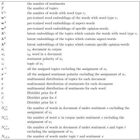
Table 3.1Notation used in this paper
S the number of sentiments
T the number of topics
Vri the number of words with word type r
i
wri pre-trained word embeddings of the words with word type r
i wA pre-trained word embeddings of aspect-words
wE pre-trained word embeddings of specific opinion-words
λri latent embeddings of the topics which contain the words with word type r
i
λA latent embeddings of the topics which contain aspect-words
λE latent embeddings of the topics which contain specific opinion-words
di ith document in corpus
wi ith word in a document
si sentiment polarity of wi
zi topic ofwi
z−i all the assigned topics excluding the assignment ofw i
s−i all the assigned sentiment polarity excluding the assignment of w i θ multinomial distribution of topics for each document
π multinomial distribution of sentiments for each document δ multinomial distribution of sentiments for each word
α Dirichlet prior for θ
β Dirichlet prior for δ
γ Dirichlet prior for π
Nd,s−i the number of words in document dunder sentimentsexcluding the assignment of wi
N−i
w,s the number of word win corpus under sentiments excluding the assignment of wi
Nd,s,t−i the number of words in document dunder sentimentsand topic t excluding the assignment ofwi
Figure 3.1 The graphical model of LDA.
general opinions.
The graphical model is shown in Figure 3.1, where Nd is the number of total words in all documents. The generative process is summarized as follows:
1. For each document d, draw a topic distributionθd∼Dir(α);
2. For each topict, draw a word distribution φt∼Dir(β);
3. For each word wi in each documentd,
(a) sample a topiczi∼M ulti(θ);
(b) sample a word wi ∼M ulti(φzi);
The probability of sampling topict to wordwi in document d, is defined as:
P(zi=t|z−i, α, β) =
Nt,w−ii+β
PW
w0=1(Nt,w−i0+β)
Nd,t−i+α
PT
t0=1(Nd,t−i0+α)
(3.1)
WhereNd,t denotes the number of times the words in document dare assigned with document t,Nt,w denotes the number of times the words assigned with topict.
The probability of word wi in topictis defined as:
P(wi |t, β) =
Nwi,t+β
PW
w0=1(Nw0,t+β)
(3.2)
Figure 3.2 The graphical model of ASUM.
3.4
ASUM
In this section, I will introduce a classic sentiment-topic model, called ASUM [25], which extends LDA by inserting a sentiment layer into LDA. In addition, ASUM imposes a constraint that all words in a sentence are generated from one topic.
The graphical model of ASUM is shown in Figure 3.2, where N is the number of words and M is the number of sentences. The generative process is summarized as follows:
1. For each pair of sentimentsand topic t, draw a word distribution φs,z ∼Dir(βs);
2. For each document d,
(a) Draw the document’s sentiment distributionπd∼Dir(γ);
(b) For each sentiment s, draw an topic distribution θd,s ∼Dir(α);
(c) For each sentence,
(a) Choose a sentiment si ∼M ulti(πd);
(b) Given sentimentsi, choose a topic zi ∼M ulti(θd,si)
W
✓
Z
!
S
⇡
A
E
S*T
↵
S
D Nd V
A
E
W
Figure 3.3 Graphical model of LOT
The probability of sentiment sin document dis defined as:
πd,s=
Nd,s+γ
PS
s0=1(Nd,s0+γ)
(3.3)
The probability of topic t in documentdwith sentiment sis defined as:
θd,s,t =
Nd,s,t+β
PT
t0=1(Nd,s,t0 +β)
(3.4)
The probability of word win senti-topic is defined as:
φw,s,t=
Nw,s,t+α
PV
w0=1(Nw0,s,t0 +α)
(3.5)
3.5
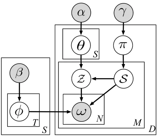
LOT Model
We now present our Latent embedding structured Opinion mining Topic model, LOT. We show the graphical representation of the model in Figure 3.3. Each node represents a variable - the shaded variables are observed, the others are hidden and must be estimated. Our notation conventions are listed in Table 4.1. Our model is a generative model and the generative process for our model proceeds as follows:
1. For each document d, draw a sentiment distributionπd∼Dir(γ),
2. For each sentiment sunderd, draw a topic distributionθd,s∼Dir(α),
![Table 3.3 Example words of the opinion list created by the authors in [24]. Left column is positiveopinion words](https://thumb-us.123doks.com/thumbv2/123dok_us/1654255.1207313/53.612.156.471.108.425/table-example-words-opinion-created-authors-column-positiveopinion.webp)
