STRONG MOTION GENERATION AREA AND ASPERITY MODEL FOR
THE 2005 MW7.8 TARAPACA, CHILE, INTRA-SLAB EARTHQUAKE
Hongjun Si1, Kazuo Dan2, Dianshu Ju2, Haruhiko Torita2, and Kiyoshi Irie2
1 Principal Researcher, Seismological Research Institute Inc., Tokyo, Japan ([email protected]) 2 Senior Researcher, Ohsaki Research Institute, Inc., Tokyo, Japan
3 Research Fellow, Ohsaki Research Institute, Inc., Tokyo, Japan 2 Deputy Director, Ohsaki Research Institute, Inc., Tokyo, Japan
2 General Manager, Research Department, Ohsaki Research Institute, Inc., Tokyo, Japan
INTRODUCTION
In June 2016, the Headquarters for Earthquake Research Promotion of Japan published a procedure (called the Recipe) for prediction of ground motions from intra-slab earthquakes. The Recipe has been validated for intra-slab earthquakes in Japan. However, it has not been well investigated for the intra-slab earthquakes outside Japan, except for the 1986 Vrancea Romania earthquake which were investigated by Ju et al. (2018).
In this study, we investigate the applicability of the Recipe to the 2005 M7.8 Tarapaca Chilean intra-slab earthquake as another example for the intra-slab earthquakes outside Japan. For the purpose, firstly, we set up fault models for the 2005 Tarapaca, Chile, earthquake in accordance with the procedure of the Recipe for evaluating the fault parameters. Then, we simulated strong ground motions for the fault models using empirical Green’s function method (EGFM) and compared them with those of the observed records.
METHOD
In order to investigate the applicability of the Recipe to the 2005 M7.8 Tarapaca, Chile, intra-slab earthquake, we forward modelled the strong motion generation area (SMGA) to reproduce the observed seismic waveform using the empirical Green’s function method. In this process, the corner frequency for the large earthquake and small earthquake, the parameters of N and C associated with the ratio of the Fourier spectra of the long-period motions (CN3) and the ratio of the Fourier spectra of the short-period motions
(CN) for the large to small events were estimated based on the source spectral fitting method proposed by Miyake et al. (1999). In the method, the parameters are derived by fitting the observed source spectral ratio between the large and small earthquake to the theoretical omega-square source spectral ratio. Then, an asperity model was assumed based on the Recipe, and it was used to reproduce the observations.
OVERVIEW OF THE PROCEDURE FOR EVALUATING FAULT PARAMETERS FOR PREDICTING STRONG GROUND MOTIONS
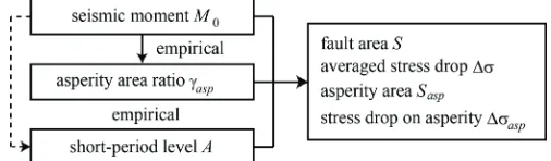
Figure 1. Official procedure of evaluating fault parameters of intra-slab earthquakes for strong motion prediction by the Headquarters for Earthquake Research Promotion (2016).
Given the size of the target earthquake, which can also be expressed by the seismic moment M0,
the short-period level A and the ratio of the asperity area to the area of the entire fault γasp can be calculated
using equations (1) to (3):
⋅ 2 = × 10× × 7 ⋅ 1/3
0
[N m/ s ] 9.84 10 ( 10 [N m]) ,
sasatani
A M (1)
−
= × × × ⋅
asasatani
S 2 16 M 7 2/3
0
[km ] 1.25 10 ( 10 [N m]) , (2)
= =
asp asp sasatani asasatani
γ S S A2 S2 π β4 4M2
0
/ (16 ) / (49 ). (3)
Here, Eq. (1) is an empirical relation between seismic moment M0 and short-period level A by
Sasatani et al. (2006). Eq. (2) is an empirical relation between seismic moment M0 and asperity area Sasp by
Sasatani et al. (2006). Finally, γasp is derived by Eq. (3) from Eq. (1) and Eq. (2).
Once the seismic moment M0, the short-period level A, and the asperity area ratio γasp are known,
the area of the entire fault S, the average stress drop Δσ, the stress drop on asperity Δσasp, and the asperity
area Sasp can be calculated using the following equations (4) to (6):
Δσ M S π 1.5 0
(7 / 16) / ( / ) ,
= (4)
=
asp asp
Δσ ( /S S ) ,Δσ (5)
= asp asp
A 4πβ2(S / )π 1/2Δσ . (6)
Here, Eq. (4) is a relation between fault area S, seismic moment M0, and average stress drop Δσ,
and it is derived from the circular crack equation by Eshelby (1957). Eq. (5) is a general formula for asperity models by Madariaga (1979). Although Eq. (6) is an empirical formula by Brune (1971) for the circular crack model, Boatwright (1988), using dynamic rupture simulations, demonstrated that the formula can be applied to asperity models.
The short-period level A for the target earthquake can be calculated from the empirical relation between seismic moment and short-period level expressed by Eq. (1), or can be referred to the value of the short-period level estimated for past intra-slab earthquakes in the region of interest.
SIMULATION OF STRONG MOTION FOR THE 2005 TARAPACA, CHILE, EARTHQUAKE
Setting up source model for the 2005 Tarapaca, Chile, earthquake
recording station discussed in this section. Figure 3 shows the acceleration waveform of the recordings at Pica station for the mainshock and aftershock.
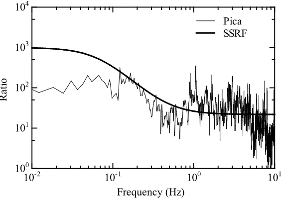
Based on the source spectral fitting method proposed by Miyake et al. (1999), we estimate parameters of N and C required for EGFM. In the analysis, firstly the ratios of Fourier spectra of recordings at Pica during the mainshock (O(f)) and aftershock (o(f)) corrected for the geometrical and anelastic attenuation are calculated as shown in right side of Eq. (7), where, R is source distance, and Qs(f) is quality factor and a value of 200 was used. Since the site effects are cancelled during the calculation, the ratio shown in Eq. (7) represents the source spectral ratio, and can be fitted by the theoretical source spectral ratio as shown in Eq. (8) based on the omega-squared source model of Brune (1970, 1971). Figure 4 shows the average source amplitude spectral ratio of two horizontal components, and the fitted theoretical source spectral ratio based on Eq. (8). By fitting Eq. (8) to the observed spectral ratio, the corner frequencies for mainshock and aftershock are estimated as fcm=0.07 and fcs=0.46Hz, respectively. Then the parameters of N and C are estimated as 7 and 3 based on Eq. (9) and (10), respectively.
−π
−π 1
( ) / exp( / ( )
( ) .
1
( ) ( ) / exp( / ( )
S S
S S
O f fR Q f V
S f = R
s f O f fR Q f V
R
(7)
+ +
cs
cm
M f f
SSRF f =
m f f
2 0
2 1 ( / )
( ) .
1 ( / ) (8)
cs
cm f N=
f . (9)
cs
cm M f
C= (
m f 3
0 ) . (10)
Figure 3. Waveforms for mainshock (left) and aftershock (left) at Pica station during the 2005 Tarapaca, Chile, earthquake.
Figure 4. Source Fourier spectral ratio of the 2005 Tarapaca, Chile, earthquake, estimated based on the recordings of mainshock and aftershock at Pica station.
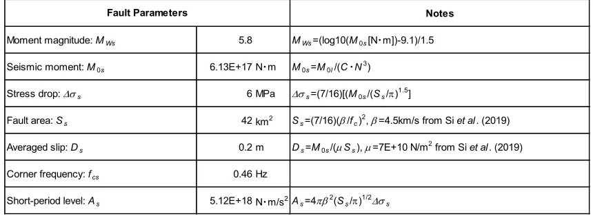
Based on the above information, we set up the asperity model for the 2005 Tarapaca, Chile, intra-slab earthquake. For the purpose, we adopted four source parameters from the previous results, including the moment magnitude of the target event MWl =7.8, the corner frequency of the small event fcs=0.46 Hz, subfault division number for the target-event fault plane N=7, and stress drop ratio between the target and small events C=3. Based on these four parameters, we determined the fault parameters for the target and small events.
Firstly, we calculated the seismic moment of the target event M0l from the moment magnitude MWl using equation (11) by Kanamori (1977):
Wl M l
M 1.5 9.1
0[N m] 10⋅ = + . (11)
Then, from the seismic moment of the target event M0l, we calculated the remaining five of the six main fault parameters, which were mentioned in the previous section, in accordance with the Recipe for strong ground motion prediction for intra-slab earthquakes by HERP (2016).
In order to estimate the short-period level of the target event Al, firstly we determined the short-period level for the small event As. Using parameters of C and N values estimated previously, the ratio of M0l /M0s was calculated using Eq. (12) and then the seismic moment of the small event M0s was also calculated:
EW -100 -50 0 50 100
Time (s)
A cc el er a tio n( cm /s 2) NS
0 10 20 30 40 50 60 70 80 90 100 -100 -50 0 50 100 EW -1000 -500 0 500 1000
Time (s)
A cc el er a tio n( cm /s 2) NS
0 10 20 30 40 50 60 70 80 90 100 -1000 -500 0 500 1000 Frequency (Hz) Ra tio Pica SSRF
10-2 10-1 100 101
100
101
102
103
= 3 =
0l / 0s 1029.
M M CN (12)
Assuming Brune’s (1970) ω-2 model, the total fault area Ssand the stress drop Δσs of the small event
can be calculated from the corner frequency of equation (13) and the circular-crack stress drop of equation (14):
= =
cs s
f β (7 / 16) /S 0.46Hz, (13)
s s s
Δσ M S π 1.5 0
(7 / 16) / ( / ) .
= (14)
Next, using the values of the fault area Ss and the stress drop Δσs of the small event, the short-period level of the small event As was calculated from Eq. (15):
s s s
A =4πβ2( / )S π 1/2Δσ . (15)
Once the short-period level of the small event As was found, the short-period level of the target event was computed by the following Eq. (16):
= =
/ 21.
l s
A A CN (16)
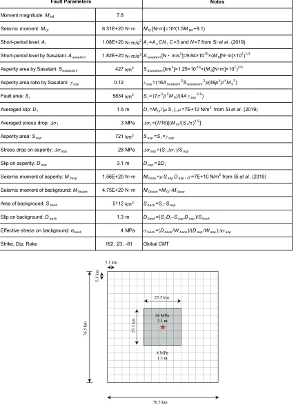
From the seismic moment M0l and the short-period level A of the target event, we calculated the asperity area ratio (ratio of the asperity area to the total fault area) γasp, the fault area Sl, the average stress drop Δσl, the stress drop on the asperity Δσasp, and the asperity area Sasp.
Furthermore, the averaged slip of the target event Dl was calculated using the following Eq. (17):
l l l
M0 =μD S. (17)
Here, the value for the shear modulus μ is equal to 7E+10 N/m2.
The averaged slip on the asperity Dasp is 2 times of averaged slip over the fault:
= ×2 .
asp l
D D (18)
Finally, the slip and the effective stress on the background area were calculated using equations (19) and (20):
=( − ) / ( − ),
back l l asp asp l asp
D D S D S S S (19)
=( / ) / ( / )⋅ .
back back back asp asp asp
σ D W D W Δσ (20)
Here, we assumed that the width of the background area is equal to the width of the fault Wback=Wl and that the asperity is square, i.e. Wasp=sqrt (Sasp).
Reproducing ground motions for the 2005 Tarapaca, Chile, earthquake
The synthetic ground motions were generated by using the empirical Green’s function method of Dan et al. (1989). The strong ground motions were calculated at one station, Pica. The location of the station with respect to the asperity model of the 2005 Tarapaca, Chile, earthquake (the target event) are shown in Figure 2. The rupture was assumed to initiate at the centre of the fault area, and the rupture velocity was taken to be VR=0.72β (here, β is the S-wave velocity) according to Geller (1976). Here, we assumed that fmax of the target event is the same as that of the small event (EGF),15Hz.
The synthetic ground motions and the pseudo-velocity response spectra computed for Pica station are plotted in Figure 3. In Figures 3(a) to 3(c), the black waveforms are the acceleration records of the small event (EGFs), the green waveforms are the synthetics calculated in this study, and the blue waveforms are the acceleration records of the target event. The peak values of the synthetic acceleration waveforms in three directions are much larger than those of the records. Figures 3(d) to 3(f) are the pseudo-velocity response spectra with 5% damping. In the period range between 0.05 to 0.2 seconds, the synthetic response spectra overpredict the recorded ones,
However, at periods longer than 0.2 seconds the synthetic response spectra reproduce the recorded ones well. The reason for the overprediction at periods shorter than 0.2s might be the effect of fmax caused by the source (Papageorgiou and Aki, 1983) or the nonlinear soil behaviour (Anderson and Hough, 1984). Therefore, we assumed that the fmax of the target event is 5Hz for the NS and EW components and 7Hz for the UD component instead of 15Hz, and then corrected the fmax from 15Hz to 5Hz or 7Hz. In Figures 3(a) to 3(f), the red plots are the revised synthetics. The results of the synthetic ground motions in NS, EW, and UD directions are quite similar to the records.
CONCLUSION
We examined the applicability of the Recipe for prediction of ground motions from intra-slab earthquakes by the Headquarters for Earthquake Research Promotion of Japan to intra-slab earthquakes outside Japan on the examples of the Chilean earthquake. We constructed the asperity models for the 2005 Tarapaca, Chile, earthquake according to the Recipe and generated synthetic ground motions using the empirical Green’s function method. The resultant synthetics waveforms reproduced the records well.
Table 1: Fault parameters of the crack model for the EGF event of the 2005 Tarapaca, Chile, earthquake.
Notes
Moment magnitude: MWs 5.8 MWs=(log10(M0s[N・m])-9.1)/1.5
Seismic moment: M0s 6.13E+17 N・m M0s=M0l/(C・N3)
Stress drop: ∆σs 6 MPa ∆σs=(7/16)[(M0s/(Ss/π)1.5]
Fault area: Ss 42 km2 Ss=(7/16)(β/fc)2, β=4.5km/s from Si et al. (2019)
Averaged slip: Ds 0.2 m Ds=M0s/(µSs), µ=7E+10 N/m2 from Si et al. (2019)
Corner frequency: fcs 0.46 Hz Si et al. (2019)
Short-period level: As 5.12E+18 N・m/s2As=4πβ2(Ss/π)1/2∆σ
Table 2: Fault parameters of the asperity model for the 2005 Tarapaca, Chile, earthquake.
Figure 5. Asperity model for the 2005 Tarapaca, Chile, earthquake (red star: hypocenter).
Notes
Moment magnitude: MWl 7.8 Si et al. (2019)
Seismic moment: M0l 6.31E+20 N・m M0l[N・m]=10^(1.5MWl+9.1)
Short-period level: Al 1.08E+20 N・m/s2Al=AsCN, C=3 and N=7 from Si et al. (2019)
Short-period level by Sasatani: Asasatani 1.82E+20 N・m/s2Asasatani[N・m/s2]=9.84×1010×(M0[N・m]×107)1/3
Asperity area by Sasatani: Sasasatani 427 km2 S
asasatani[km2]=1.25×10⁻¹⁶×(M0[N・m]×107)2/3
Asperity area ratio by Sasatani:γasp 0.12 γasp=(16Asasatani2Sasasatani2)/(49p4β4M02)
Fault area: Sl 5834 km2 Sl=(7π2β2M0)/(4Aγasp0.5)
Averaged slip: Dl 1.5 m Dl=M0l/(µSl), µ=7E+10 N/m2 from Si et al. (2019)
Averaged stress drop: ∆σl 3 MPa ∆σl=(7/16)[(M0l/(Sl/π)1.5]
Asperity area: Sasp 721 km2 Sasp=Sl×γasp
Stress drop on asperity: ∆σasp 28 MPa ∆σasp=(Sl∆σl)/Sasp
Slip on asperity: Dasp 3.1 m Dasp=2Dl
Seismic moment of asperity: M0asp 1.56E+20 N・m M0asp=µSaspDasp, µ=7E+10 N/m2 from Si et al. (2019)
Seismic moment of background: M0back 4.75E+20 N・m M0back=M0l-M0asp
Area of background: Sback 5112 km2 Sback=Sl-Sasp
Slip on background: Dback 1.3 m Dback=(SlDl-SaspDasp)/Sback
Effective stress on background: σback 4 MPa σback=(Dback/Wback)/(Dasp/Wasp)∆σasp
Strike, Dip, Rake Global CMT
Fault Parameters
(a) NS accelerations (b) EW accelerations (c) UD accelerations
(d) NS response spectra (e) EW response spectra (f) UD response spectra
Figure 6. Comparison of the synthesized results by the asperity model with the recordings at Pica in the 2005 Tarapaca, Chile, earthquake.
REFERENCES
Anderson, JG and Hough SE (1984), “A model for the shape of the Fourier amplitude spectrum of acceleration at high frequencies”, Bulletin of the Seismological Society of America, 74 (5), pp.1969-1993.
Boatwright J (1988), “The seismic radiation from composite models of faulting”, Bulletin of the Seismological Society of America, 78(2): 489-508.
Brune JN (1970), “Tectonic stress and the spectra of seismic shear waves from earthquakes”, Journal of Geophysical Research, 75(26): 4997-5009.
Dan K, Watanabe T, and Tanaka T (1989), “A semi-empirical method to synthesize earthquake ground motions based on approximate far-field shear-wave displacement”, Journal of Structural and Construction Engineering (Transactions of the Architectural Institute of Japan), 396: 27-36 (in Japanese).
Eshelby JD (1957), “The determination of the elastic field of an ellipsoidal inclusion, and related problems”, Proceedings of the Royal Society of London, Series A, 241: 376-396.
Geller RJ (1976), “Scaling relations for earthquake source parameters and magnitudes”, Bulletin of the Seismological Society of America, 66(5): 1501-1523.
Headquarters for Earthquake Research Promotion (2016), “Strong ground motion prediction method for earthquakes with specified source faults ("Recipe")” (in Japanese) .
Hayes, G. (2005). “Preliminary Finite Fault Results for the Jun 13, 2005 Mw 7.7 -20.0100, -69.2400 Earthquake (Version 1),” https://earthquake.usgs.gov/earthquakes/eventpage/usp000dsw1#finite-fault (last access: 20180830).
Ju, D., Dan K. Dorjpalam S. and Torita, H. (2018). “Applicability of Procedure for Evaluating Fault Parameters of Intra-Slab Earthquakes by HQERP, Japan, to Romanian earthquakes,” Proc., 16th European Conference on Earthquake Engineering, Thessaloniki, Greece.
Madariaga R (1979), “On the relation between seismic moment and stress drop in the presence of stress and strength heterogeneity”, Journal of Geophysical Research, 84(B5): 2243-2250.
Miyake, H., T. Iwata, and K. Irikura (1999). “Strong ground motion simu- lation and source modeling of the Kagoshima-ken Hokuseibu earth- quakes of March 26 (MJMA 6.5) and May 13 (MJMA 6.3), 1997,
using empirical Green's function method”, Zisin, 51, 431-442 (in Japanese with English abstract). Papageorgiou AS and Aki K (1983), “A specific barrier model for the quantitative description of
inhomogeneous faulting and the prediction of strong ground motion II. Application of the model”, Bulletin of the Seismological Society of America, 73(4), pp.953-978.